x – x

Standardization conversion formula

t = ––––

σx

Standard Umrechnungsformel


Formule de conversion de standardisation


Fórmula de conversión de estandarización


Fórmula de conversão padronizada


Formula di conversione della standardizzazione


Standaardisering omzettingsformule


Standard átváltási képlet


Vzorec pro přepočet rozdělení


Omvandlingsformel för standardisering


Normituksen konversiokaava


îÓÏÛ· Òڇ̉‡ÚËÁÓ‚‡ÌÌÓ„Ó ÔÂÓ·‡ÁÓ‚‡ÌËfl


Omregningsformel for standardisering

Rumus penukaran pemiawaian

Rumus konversi standarisasi

Coâng thöùc bieán ñoåi chuaån hoùa

m(2-VLE)


a1x + b1y = c1


D


=

a1 b1


a2x + b2y = c2


a2

b2


2x + 3y = 4

m20


2 ®3 ®4 ®


5x + 6y = 7

5 ®6 ®7


x = ?

®[x]


–1.

y = ?

®[y]

2.

det(D) = ?

®[det(D)]


–3.


m(3-VLE)


a1x + b1y + c1z = d1


a1 b1 c1


a2x + b2y + c2z = d2


D

=

a2 b2 c2


a3x + b3y + c3z = d3


a3 b3 c3


m21

x + y z = 9 1 ®1 ®1 ±®9 ®

6x + 6y z = 17 6 ®6 ®1 ±®17 ® 14x – 7y + 2z = 42 14 ®7 ±®2 ®42

x = ?

®[x]

3.238095238

y = ?

®[y]

–1.638095238

z = ?

®[z]

–7.4

det(D) = ?

®[det(D)]

105.


m(QUAD, CUBIC)


m22


3x2 + 4x – 95 = 0 3 ®4 ®±95


x1 = ?

®

5.

x2 = ?

®

–6.333333333


5.


m23


5x3 + 4x2 + 3x + 7 = 0 5 ®4 ®3 ®7


x1 = ?

®

–1.233600307

x2 = ?

®

0.216800153

y

• • • •

@{8 Ö70 +12

Ö25


A


=[r]

18.5408873

r1

r


@≠[θ]

42.76427608


θ

B

θ1

θ2

r2


x


r1 = 8, θ1 = 70° r2 = 12, θ2 = 25°

r = ?, θ = ?°

(1 + i)

@}1 +Ü=

1.

@{[r]

1.414213562

r = ?, θ = ?°

@≠[θ]

45.


@}(2 -3Ü)L

(2 – 3i)2 =

=[x]

–5.


@≠[y]

12. i

1

(1 +Ü)@•=[x] 0.5

—— =

@≠[y]

0.5 i

1 + i

CONJ(5+2i) =

∑0(5 +2 Ü)=[x] 5.


@≠[y]

2. i

m(MAT)


m4


1 2


matA


]2 k2 k1 k2 k


3 4


3 k4 k


3 1


matB


ª∑20


]2 k2 k


2 6


3 k1 k2 k6 k


ª∑21


matA matB =


7


13


ª∑00*∑01=


17 27


matA–1=


–2

1


ª∑00@•=


1.5 –0.5


1 2 0


ª∑30∑00

dim(matA,3,3) =

3 4 0


0 0 0


@,3 @,3 )=


5 5 5


ª∑315 @,

fill(5,3,3) =

5 5 5


3 @,3 )=


5 5 5


cumul matA =


1 2


ª∑32∑00=


4 6


aug(matA,matB) =


1 2 3 1


ª∑33∑00


3 4 2 6


@,∑01)=


1 0 0


identity 3 =

0 1 0


ª∑343 =


0 0 1


rnd_mat(2,3)


ª∑352 @,3 )=


det matA = –2


ª∑40∑00=


trans matB =

3 2


ª∑41∑01=

1 6


L1: {1 3}


mat list L2: {3 2}

ª∑5

m(LIST)


m5

2, 7, 4 L1

]3 k2 k7 k4 k

–3, –1, –4 L2

ª∑20

]3 k


±3 1 4 k ª∑21

L1+L2 = {–1 6 0}ª∑00+∑01=

sortA L1 = {2 4 7}ª∑30∑00=

sortD L1 = {7 4 2}ª∑31∑00=

• • • •

stdDv L1 = 2.516611478 ª∑46∑00=

vari L1 = 6.333333333 ª∑47∑00=

o_prod(L1,L2) = {–24 –4 19} ª∑48∑00 @,∑01)=

i_prod(L1,L2) = –29 ª∑49∑00 @,∑01)=

abs L2 = 5.099019514 ª∑4A∑01=


2 –3


list matA matA:


7 –1


ª∑6


4 –4


Function


Dynamic range

Funktion


zulässiger Bereich

Fonction


Plage dynamique

Función


Rango dinámico

Função


Gama dinâmica

Funzioni


Campi dinamici

Functie


Rekencapaciteit

Függvény


Megengedett számítási tartomány

Funkce


Dynamický rozsah

Funktion


Definitionsområde

Funktio


Dynaaminen ala

îÛÌ͈Ëfl


ÑË̇Ï˘ÂÒÍËÈ ‰Ë‡Ô‡ÁÓÌ

Funktion


Dynamikområde

Fungsi


Julat dinamik

Fungsi


Kisaran dinamis

Haøm soá


Giôùi haïn Ñoäng


DEG:

x < 1010


(tan x : x 90 (2n–1))*

sin x, cos x,


RAD:


π

1010


x < —–

tan x


180


π


(tan x : x (2n–1))*


10

2


10


GRAD: x < —–

10


9


(tan x : x 100 (2n–1))*

sin–1x,cos–1x


x 1


tan–1x, 3¿x


x < 10100


In x, log x


10–99x < 10100


y > 0: –10100< x log y < 100

yx


y = 0:

0 < x < 10100


y < 0: x = n


1


(0 < l x l < 1: — = 2n–1, x 0)*,


x


–10100< x log y < 100


1


y > 0: –10100< — log y < 100 (x 0)


x


y = 0:

0 < x < 10100

x¿y


y < 0: x = 2n–1


1


(0 < x < 1 : — = n, x 0)*,


1

x


–10100< — log y < 100


x


ex


–10100< x 230.2585092

10x


–10100< x < 100


sinh x, cosh x,


x 230.2585092


tanh x


sinh–1x


x < 1050


cosh–1x


1 x < 1050


tanh–1x


x < 1


x2


x < 1050


x3


x < 2.15443469 1033


¿x


0 x < 10100


x–1


x < 10100 (x 0)


n!


0 n 69*


nPr


0 r n 9999999999*


n!


100


—— < 10


(n-r)!


0 r n 9999999999*


@≠

+ 1.043018296 i

x3 = ?

®

0.216800153

dim(L1,5) = {2 7 4 0 0}

ª∑32∑00 @,5 )=

nCr

0 r 69

n!


—— < 10100


(n-r)!

@≠

1.043018296 i

m(CPLX)

m3

(12–6i) + (7+15i) – 12 -6 Ü+7 +15 Ü-

(11+4i) =

(11 +4 Ü)=[x] 8.


@≠[y]

+ 5. i


@≠[x]

8.


6(7–9i)

6 *(7 -9 Ü)*

(–5+8i) =

(5 ±+8 Ü)=[x] 222.


@≠[y]

+ 606. i

16(sin30°+

16 *(s30 +


icos30°)÷(sin60°+

Üu30 )/(s60 +

icos60°)=

Üu60 )=[x]

13.85640646


@≠[y]

+ 8. i

• • • •

fill(5,5) = {5 5 5 5 5}

ª∑335 @,

5 )=


cumul L1 = {2 9 13}

ª∑34∑00=


df_list L1 = {5 –3}

ª∑35∑00=

aug(L1,L2) = {2 7 4 –3 –1 –4} ª∑36∑00 @,∑01)=

min L1 = 2

ª∑40∑00=


max L1 = 7

ª∑41∑00=

mean L1 = 4.333333333 ª∑42∑00=

med L1 = 4

ª∑43∑00=


sum L1 = 13

ª∑44∑00=


prod L1 = 56

ª∑45∑00=

• • • •

DEG, D°M’S

0°0’0.00001” x < 10000°

x, y r, θ


x2 + y2 < 10100


0 r < 10100


DEG:

θ < 1010


r, θ → x, y

RAD:

θ

π

1010

< —–


180


GRAD : θ

10

10


< — 10


9


DRG

DEGRAD, GRADDEG: x < 10100


π

98


RADGRAD: x < —

10


2


(A+Bi)+(C+Di)

A + C < 10100, B + D < 10100

(A+Bi)–(C+Di)

A – C < 10100, B – D < 10100

(A+Bi)(C+Di)

(AC – BD) < 10100


(AD + BC) < 10100


• • • •

Page 7
Image 7
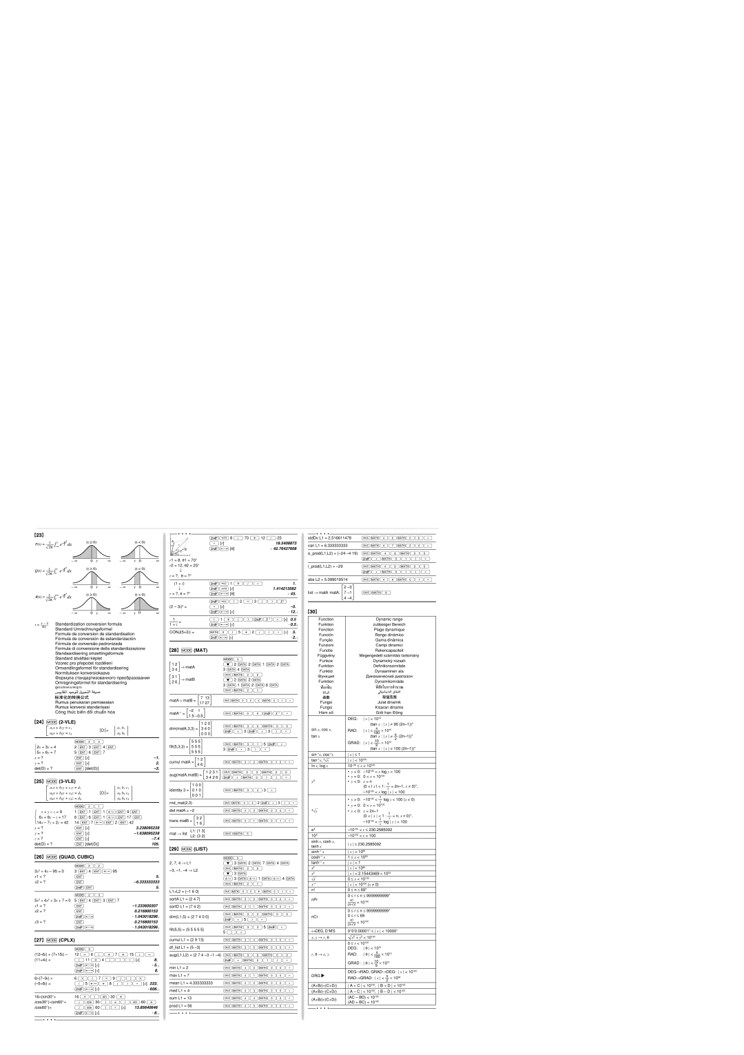
Sharp EL-506W, EL-546W manual M2-VLE, M3-VLE, MQUAD, Cubic, Mmat, Mlist, Mcplx

EL-506W, EL-546W specifications

The Sharp EL-506W and EL-546W are advanced scientific calculators designed to meet the needs of students, professionals, and anyone requiring reliable mathematical calculations. Both models feature a blend of user-friendly design and sophisticated technology, making them ideal tools for educational and professional use.

The Sharp EL-506W is equipped with a wide array of functionalities, boasting over 300 scientific functions including standard calculations, statistical analyses, and trigonometric computations. One of its key features is the two-line display that allows users to view both the input and the result simultaneously, enhancing clarity and reducing the likelihood of input errors. It also includes a function for creating equations, enabling seamless entry and editing of mathematical expressions.

On the other hand, the EL-546W offers a broader range of features, with more than 400 functions covering everything from algebraic calculations to calculus. It supports complex number calculations and provides a unique "Math" display mode that shows results in traditional mathematical notation, making it highly suitable for more advanced calculations. The EL-546W also includes built-in memory, which allows users to store and recall calculations effortlessly.

Both calculators employ Sharp's proprietary "Dual-Text" technology, which enables users to perform operations in a clear and logical manner. The ergonomic design of these models ensures comfort during extended use, with a layout that places frequently used buttons within easy reach. The durable construction of the calculators enhances their longevity in various environments, making them reliable companions for daily use.

In terms of power efficiency, the EL-506W and EL-546W are designed to maximize battery life. They feature an automatic power-off function that preserves energy when the calculators are not in use, ensuring that users can rely on them when needed most.

Overall, the Sharp EL-506W and EL-546W stand out for their robust feature sets, user-friendly interfaces, and versatility in handling a diverse range of mathematical functions. Whether you're solving complex equations or performing routine calculations, these scientific calculators provide the precision and reliability necessary for any mathematical task.