Appendix E a Detailed Look at f | HP 15c Scientific specification

252 Appendix E: A Detailed Look at f

The graph is a spike very close to the origin. (Actually, to illustrate f(x) the width of the spike has been considerably exaggerated. Shown in actual scale over the interval of integration, the spike would be indistinguishable from the vertical axis of the graph.) Because no sample point happened to discover the spike, the algorithm assumed that f(x) was identically equal to zero throughout the interval of integration. Even if you increased the number of sample points by calculating the integral in i 9, none of the additional sample points would discover the spike when this particular function is integrated over this particular interval. (Better approaches to problems such as this are mentioned at the end of the next topic, Conditions That Prolong Calculation Time.)

You've seen how the f algorithm can give you an incorrect answer when f(x) has a fluctuation somewhere that is very uncharacteristic of the behavior of the function elsewhere. Fortunately, functions exhibiting such aberrations are unusual enough that you are unlikely to have to integrate one unknowingly.

Functions that could lead to incorrect results can be identified in simple terms by how rapidly it and its low-order derivatives vary across the interval of integration. Basically, the more rapid the variation in the function or its derivatives, and the lower the order of such rapidly varying derivatives, the less quickly will the f algorithm terminate, and the less reliable will the resulting approximation be.

Image 252

HP 15c Scientific manual Appendix E a Detailed Look at f

Contents

HP-15C Owner’s Handbook HP Part Number 00015-90001 Edition 2.4, Sep Legal Notice Introduction Contents Contents Display and Continuous Memory Program Editing Program Branching and Controls Subroutines Indirect Display Control Calculating With Complex NumbersCalculating With Matrices Numerical Integration Contents Appendix a Error Conditions Appendix C Memory AllocationAppendix D a Detailed Look at Appendix E a Detailed Look at f Contents Appendix F Batteries Function Summary and IndexProgramming Summary and Index Subject Index HP-15C Problem Solver Quick Look at Manual Solutions To Compute Keystrokes Display Programmed Solutions Keystrokes Display KeystrokesDisplay 001-42,21,11002 003 004 005 006 007 008 009 8313 300.51 HP-15C a Problem Solver Part l HP-15C Fundamentals Power On and Off Getting StartedKeyboard Operation Section Prefix Keys Changing SignsKeying in Exponents I O m ´ P I l F T s ? t H b Clear Keys Display Clearing ` and − Digit entry not terminatedClears only the last digit Calculations One-Number FunctionsTwo-Number Functions 6532 17 + 26.0000 22.0000 500013.0000 78.0000 Numeric Functions Number Alteration Functions One-Number Functions General Functions Trigonometric Operations Time and Angle ConversionsPressing Calculates Degrees/Radians Conversions 7069Radians 40.5000 Logarithmic Functions Hyperbolic Functions Power Function Two-Number FunctionsPercentages To Calculate Keystrokes Display Polar and Rectangular Coordinate Conversions Enters the base number the priceCalculates 3% of $15.76 the tax Polar Conversion. Pressing Keystrokes Display Automatic Memory Stack Last X, and Data Storage Automatic Memory Stack Stack ManipulationAutomatic Memory Stack Registers Always displayed Stack Manipulation Functions Memory Stack, Last X, and Data StorageLost Lost Last X Register and K 287.000022.2481 12.9000 Calculator Functions and the Stack 13.9 +20.6475 Order of Entry and the v Key +15 X15 Nested Calculations 7 +65.0000 69.0000 Arithmetic Calculations With Constants 5 ‛15 Keys Keystrokes Display Growth factor 1000000 Storage Register Operations Storing and Recalling Numbers322.5000 520.8750 Clearing Data Storage Registers Storage and Recall Arithmetic For storage arithmetic For recall arithmetic Problems Overflow and Underflow24 l-0 15.0000 Memory Stack, Last X, and Data Storage Statistics Functions Probability Calculations60.0000 Random Number Generator 270,725.00005764 3422 Accumulating Statistics Registers Register Contents 20.00 40.00 60.00 80.00 Kg per hectare Metric tons per Hectare, y20 z 61v 40 z 7.21 60 z 7.78 80 z l Σy2 Correcting Accumulated Statistics 20 w 20 z Mean Standard Deviation40.00 Linear Regression 31.62Standard deviation about the mean nitrogen Application Linear Estimation and Correlation Coefficient Statistics Functions Other Applications 70 ´j Display Continuous Memory Display ControlFixed Decimal Display Scientific Notation Display Engineering Notation Display234568 234567 Round-Off Error Special DisplaysMantissa Display Annunciators Error Display Digit Separators12,345.67 12.345.6700 Low-Power Indication Continuous MemoryStatus Resetting Continuous Memory Page Part ll HP-15C Programming Programming Basics MechanicsCreating a Program Loading a Program Programming Basics ´b a Intermediate Program Stops Running a Program002 003 004 005 006 007 008 How to Enter Data 300.51 300.51 ´A Program Memory Radius, r Height, h Base Area Volume Surface Area Totals 002 004 005007-44,40 010 Or G a Further Information Program InstructionsInstruction Coding Memory Configuration Keycode 25 second row, fifth key Initial Memory Configuration 60 ´ m% Program Boundaries ´ m %19 ´ m% 19.0000 Unexpected Program Stops Abbreviated Key Sequences´bA ´b3 End of memory User Mode Polynomial Expressions and Horners Method¤ @ y ∕ LOG % Nonprogrammable Functions 001-42,21,12002 003 004 005 006 007 008 009 0000 12,691.0000 Problems Program Editing Moving to a Line in Program Memory Examples Deleting Program LinesInserting Program Lines Or use Â Single-Step Operations Line Position ÂholdRelease Result Insertions and Deletions Initializing Calculator Status Interest + i nPV 1 + i n 100 270 ´bA D ´4 O0 2* O1 2÷ * ´ ´ l0 l1 ´r * n Program Branching Controls Branching Conditional Tests Test Flags  n will clear flag number n Example Branching and Looping 010-45,20 013-43,30014 016-44,40 Example Flags Formula is 002-43 004-42,21,15005-43, 4 006-42,21 Go to 250.000048.0000 10,698.3049 Looping Conditional Branching System Flags Flags 8 Program Branching and Controls Subroutines Go To Subroutine and ReturnSubroutine Execution ´b.1 Subroutine Limits 000 001- ´b9 002- R003- O0 004 ´ b.4 ´b.5 Subroutine Return Nested Subroutines Index Register Loop Control V and % Keys106 Indirect Program Control With the Index Register Program Loop ControlIndex Register Storage and Recall Index Register and Loop Control Index Register Arithmetic Exchanging the X-RegisterIndirect Branching With Indirect Flag Control With Indirect Display Format Control WithLoop Control With Counters I and e Nnnnn x x x y y 5 0 0 Start count at zero Count by twos Count up to Examples Register Operations IterationsStoring and Recalling Keystrokes Display 12.3456 Example Loop Control with e Exchanging the X-RegisterStorage Register Arithmetic Loop control number in R2 −− 011- 42012-42, 5 013- 22 Example Display Format Control 15 O64.8420 0000 50.0000 Index Register Contents Indirect Display Control Index Register and Loop Control 118 Part lll HP-15C Advanced Functions Complex Stack and Complex Mode Calculating With Complex NumbersCreating the Complex Stack 120 Deactivating Complex Mode Complex Numbers and the StackEntering Complex Numbers ´ % hold 8.0000 release Z 8 Y 7 X Keys Stack Lift in Complex Mode Manipulating the Real and Imaginary Stacks Clearing a Complex Number Or other operation Continue with any operation − 4 v Continue with any operation Entering Complex Numbers with −. The clearing functions − ´ %hold release0000 17.0000 144.0000 Entering a Real Number Followed by another number Entering a Pure Imaginary Number ´ Continue with any operation Operations With Complex Numbers Storing and Recalling Complex Numbers´ O L 2 ´ ¤x N o ∕ @ a + * ÷ y 2000 70000428 0491 Polar and Rectangular Coordinate Conversions Complex Results from Real Numbers5708 ´ % hold Release1.5708 Cos θ + i sin θ = re iθ Polar + ib = ∠ θ 8452 2981+ 3.1434 352.0000 872.00002361 4721 For Further Information Calculating With Matrices 138 Keystrokes Display Deactivates Complex Mode = A-1B Matrix Dimensions Running11.2887 2496 Dimensioning a Matrix Number Rows Columns Displaying Matrix Dimensions Changing Matrix Dimensions´mA Keystrokes l B Display Storing and Recalling Matrix Elements Storing and Recalling All Elements in Order ⎡ a Checking and Changing Matrix Elements Individually Keystrokes Display Matrix Operations Storing a Number in All Elements of a MatrixMatrix Descriptors Result Matrix Copying a Matrix One-Matrix Operations Calculating with Matrices Scalar Operations LB b Elements of Result Matrix LA a Arithmetic Operations Keystrokes Display Subtracts 1 from the elementsLB b 2 LA a 2 Matrix Multiplication = AT B Keystrokes Display l a a Solving the Equation AX = B 24 OA 240086 OA 8600 274 OB 233 OB 331 OB 120.32 OB 112.96 OB 151.36 OB ´Á Calculating the Residual Week Cabbage kg 186 141 215 Broccoli kg 116 Using Matrices in LU Form Calculations With Complex Matrices Storing the Elements of a Complex Matrix Then Z can be represented in the calculator by Pressing Transforms Into = ⎢ LA a Complex Transformations Between ZP and Z Inverting a Complex Matrix Multiplying Complex Matrices ´ a Keystrokes lA lB Display Displays descriptor of matrix a ´U lC LC lC lC lC lC lC lC ´U Solving the Complex Equation AX = B ZZ −1 AX = B 200.0000 170.0000 0372 13110437 1543 Calculating with Matrices Using a Matrix Element With Register Operations Using Matrix Descriptors in the Index RegisterMiscellaneous Operations Involving Matrices Stack Operation for Matrix Calculations Conditional Tests on Matrix Descriptors Calculating with Matrices Using Matrix Operations in a Program Summary of Matrix Functions Keystrokes Results´m a Calculates residual in result matrix For Further Information Using Finding the Roots An Equation180 Finding the Roots of an Equation Clear program memory ´b0 001-42,21002 003 005 006 007 Finding the Roots of an Equation Desired root Keystrokes ¥ ´ bA000 001-42,21,11 003 004 5000 1 e t Brings another t-valueInto X-register 200 t When No Root Is Found 000 001-42,21 002 003 004 005 Error Choosing Initial Estimates Label 003 004 005 007 X + 8008 009 6 x + 8 Finding the Roots of an Equation Using in a Program Restriction on the Use Memory Requirements Using f Numerical Integration194 002 003 004 4040 1416 7652 Begin subroutine with a label 3825 $ ÷4401 6054 Accuracy of f ´ i ´ f 8826 7091 Using f in a Program 382 Memory Requirements Error Conditions Error 0 Improper Mathematics OperationAppendix a 205 Error 1 Improper Matrix Operation Error 2 Improper Statistics Operation Error 3 Improper Register Number or Matrix Element Error 4 Improper Line Number or Label CallError 5 Subroutine Level Too Deep Error 6 Improper Flag Number Pr Error Power Error Stack Lift Last X Register Digit Entry TerminationStack Lift Appendix B Disabling Operations Enabling Operations Stack Stack Enabled. disabled 53.1301 No stack Lift Neutral OperationsAppendix B Stack Lift and the Last X Register Keys Nnn Clear u ¥ Last X Register \ k + H ∆ \ h ÷ À P* q r c ‘ / N z ∕ P\ o j Memory Allocation Memory SpaceAppendix C Registers Appendix C Memory Allocation Memory Reallocation Memory Status WM % Function Restrictions on Reallocation ´m% 1.0000 Whold 1 6419 ´ m Program Memory Automatic Program Memory Reallocation Memory Requirements for the Advanced Functions Two-Byte Program InstructionsIf executed Together Appendix C Memory Allocation Detailed Look at How WorksAppendix D 220 Appendix D a Detailed Look at Accuracy of the Root X4 = 000 1718 006 007 008 009 010-43,30 011 012-43,30 013 Interpreting Results ´ v B0681 − 45 For 0 x Test for x range Branch for x ≥3x 45x 2 + End subroutine 000.0000 Initial estimates1358 Possible root Appendix D a Detailed Look at ´ b.0 001-42,21,.0 002 003 004 005 Bring x-value into X-register007 008 009 010 013 014 015 016 017 018 10 v ´ ‛ 20 Error 0000 1250 5626 Finding Several Roots Fx = xx a3 = 002 003 004 005 006 007 6667 Same initial estimates Second rootStores root for deflation Deflated function value Deflation for third root Limiting the Estimation Time For Advanced Information Counting IterationsSpecifying a Tolerance Detailed Look at f How f WorksAppendix E 240 Accuracy, Uncertainty, and Calculation Time X = π1 0π cos4θ − x sinθ dθ 0000 1416 ´ i ´ f Keystrokes Display Return approximation to ´ Clear u HoldKeystrokes ´ i Display ´ f ´ Clear u hold 7858 7807 Uncertainty and the Display Format Functions values for example Δx = 0.5×10−n ×10m = aδx dxb = ab 0.5×10−n + m x dx 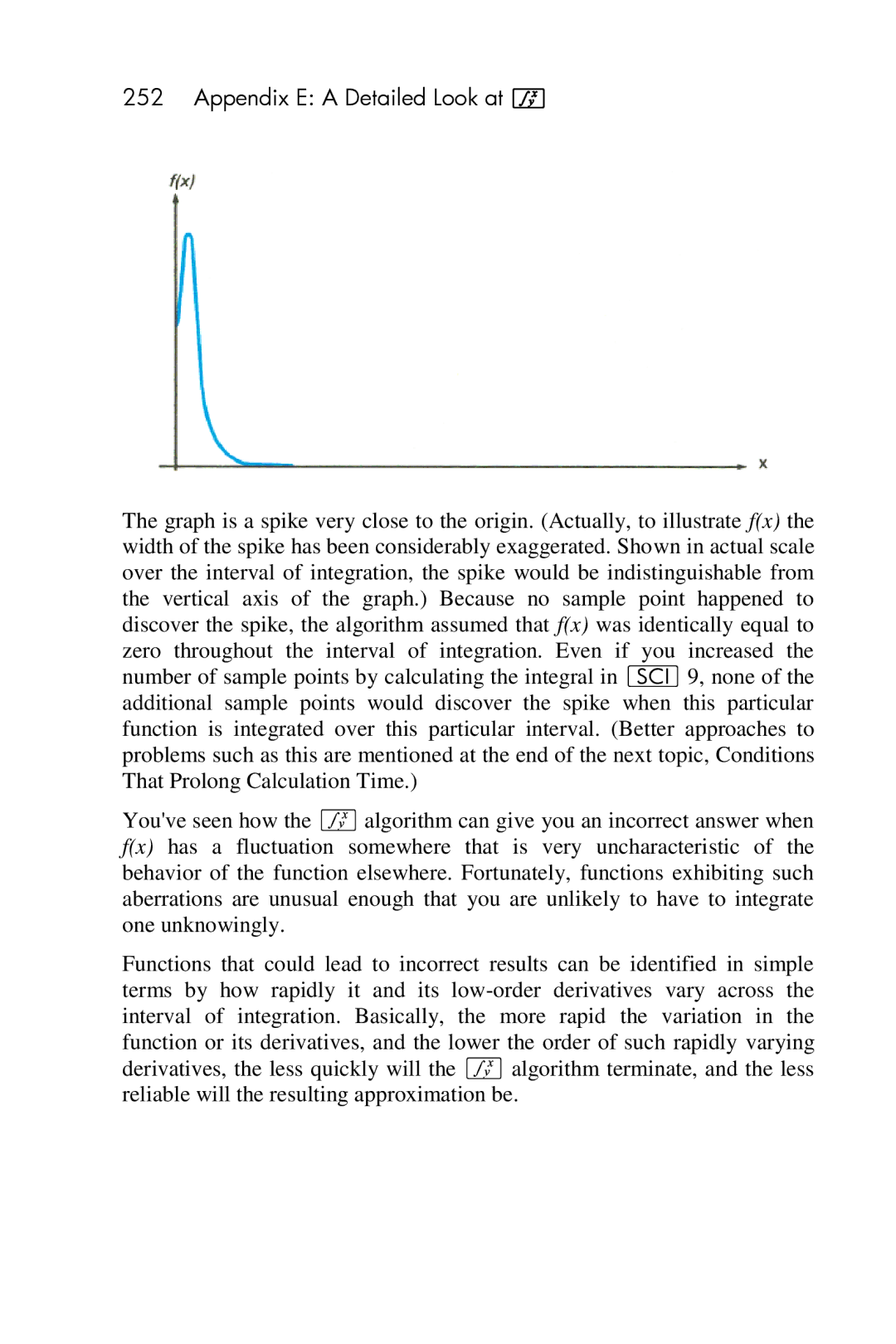Conditions That Could Cause Incorrect Results ∞ xe− xdx 001-42,21 002- 1 003 004 005 Appendix E a Detailed Look at f Appendix E a Detailed Look at f Conditions That Prolong Calculation Time Keys lower limit into Keys upper limit intoApproximation to integral Uncertainty Appendix E a Detailed Look at f Obtaining the Current Approximation to an Integral For Advanced Information Low-Power Indication Installing New BatteriesBatteries Batteries Appendix F Batteries Verifying Proper Operation Self-Tests 2.C 3.H Function Summary and Index Complex FunctionsConversions Digit Entry Display Control Index Register ControlLogarithmic Exponential Functions Mantissa. Pressing Mathematics Matrix Functions146 Number Alteration To ZP page164To XT Percentage ProbabilityStack Manipulation Clear u Statistics Storage Trigonometry Programming Summary and Index 269 Programming Summary and Index Subject Index 271 Subject Index Subject Index Subject Index Subject Index Subject Index Subject Index Subject Index Subject Index Subject Index Subject Index Subject Index Subject Index Product Regulatory Environment Information Federal Communications Commission NoticeModifications Canadian Notice Avis Canadien European Union Regulatory Notice Body number is inserted between CE