Model SR850
Page
Table of Contents
Table of Contents
Safety and Preparation for USE
Page
Reference Channel
SR850 DSP LOCK-IN Amplifier Specifications
Signal Channel
Demodulator
Displays
SR850 DSP Lock-In Amplifier
Inputs and Outputs
Analysis Functions
Command List
Variables
AUX INPUT/OUTPUT
Cursor
Mark
Math
Front Panel Controls
Setup
Print and Plot
Auto Functions
Interface
Standard Event Status Byte Error Status Byte
Status Byte Definitions
Status
Getting Started Your First Measurements
Key Types Hardkeys Softkeys Knob
Getting Started
Basic LOCK-IN
Basic Lock-in
Basic Lock-in
Basic Lock-in
Basic Lock-in
Displays and Traces
Displays and Traces
Displays and Traces
Displays and Traces
Displays and Traces
Displays and Traces
Displays and Traces
OUTPUTS, Offsets and Expands
Outputs, Offsets and Expands
Outputs, Offsets and Expands
Outputs, Offsets and Expands
Outputs, Offsets and Expands
Scans and Sweeps
Scans and Sweeps
Scans and Sweeps
Scans and Sweeps
Scans and Sweeps
Scans and Sweeps
Scans and Sweeps
Storing and Recalling Data
Using the Disk Drive
Disk Drive
Disk Drive
Disk Drive
Disk Drive
Disk Drive
Disk Drive
Storing and Recalling Settings
TEST1
AUX Outputs and Inputs
Aux Outputs and Inputs
Aux Outputs and Inputs
Aux Outputs and Inputs
Aux Outputs and Inputs
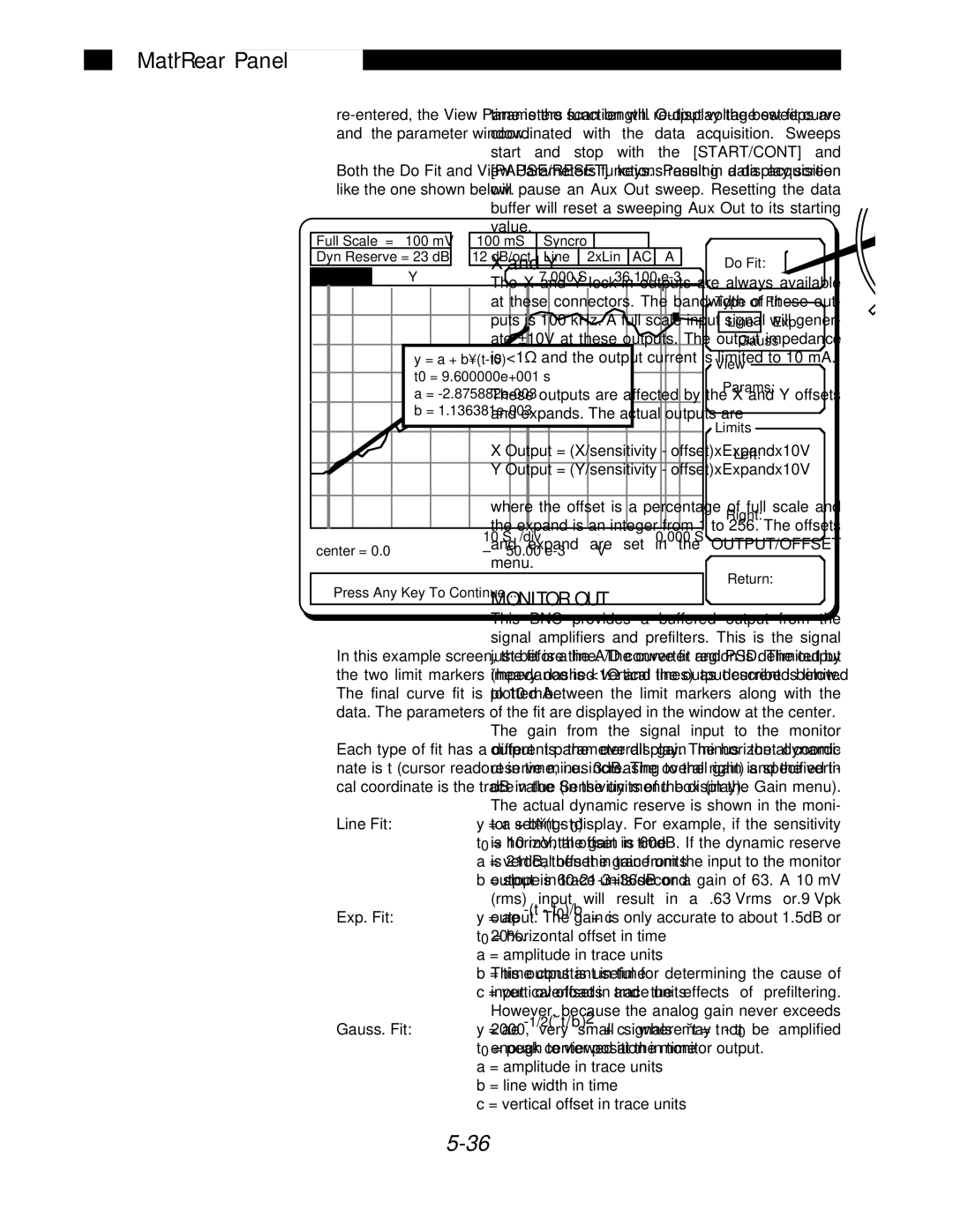
Trace Math
Trace Math
Trace Math
Right edge of the graph display. In this case
Trace Math
Trace Math
Trace Math
Trace Math
Trace Math
What is phase-sensitive detection?
SR850 Basics What is a LOCK-IN AMPLIFIER?
Why use a lock-in?
Magnitude and phase
Where does Lock-in reference come from?
All lock-in measurements require a reference signal
SR850 Basics
What does the SR850 measure?
What does a LOCK-IN MEASURE?
RMS or Peak?
Degrees or Radians?
SR850 Basics
PLL
SR850 Functional Block Diagram
Functional SR850
SR850 Basics
Reference Channel
Reference Oscillators and Phase
Phase Jitter
Reference Input
Harmonic Detection
Phase Sensitive Detectors PSDs
Digital PSD vs Analog PSD
SR850 Basics
Digital Filters vs Analog Filters
Time Constants and DC Gain
Time Constants
Synchronous Filters
DC Output Gain
What about resolution?
Long Time Constants
R and Output scales
DC Outputs and Scaling
CH1 and CH2
R Output Offset and Expand
Trace displays
Trace output scaling
SR850 Basics
SR850 Basics
What is dynamic reserve really?
Dynamic Reserve
Dynamic reserve in the SR850
Minimum dynamic reserve
Notch filters
Signal Input Amplifier and Filters
Input noise
Anti-aliasing filter
Input Impedance
Differential Voltage Connection A-B
Common Mode Signals
Input Connections
Single-Ended Voltage Connection a
Current Input
AC vs DC Coupling
Shot noise
Intrinsic Random Noise Sources
Johnson noise
Noise
SR850 Basics
Inductive coupling
External Noise Sources
Capacitive coupling
Thermocouple effects
Resistive coupling or ground loops
Microphonics
Noise estimation
Noise Measurements
How does a lock-in measure noise?
Noise
Video Display
Power Button
Front Panel
Front Panel
Signal Inputs
Ch1 & Ch2 Outputs
Front Panel
Soft Key Definitions
Default Display
Status Activity Indicators
Soft Keys
Trace 1 Trace 2 Y Trace 3 R
Screen Display
Data Traces
AI1
Single and Dual Trace Displays
Screen Display
BAR Graphs
Plot of X and Y
Signal Vector
Polar Graphs
Scale
Strip Charts
Chart Scaling
Cursor Display
Data Scrolling
Cursor
Marks
Trace SCANS, Sweeps & Aliasing
Aliasing Effects
Default Scan
Starting and Stopping a Scan
Settings & INPUT/OUTPUT Monitor Menu Display
Status Indicators
SRQ
ALT
Screen Display
Menu Keys
Keypad
Normal and Alternate Keys
Additional Menus
START/CONT and PAUSE/RESET
Keypad
Entry Keys
Mark
Cursor
Active Display
Cursor MAX/MIN
Auto Phase
Auto Setup
Auto Reserve
Help
Print to a Printer
Print to a Disk File
Local
Keypad
RS232 Connector
Power Entry Module
IEEE-488 Connector
PC Keyboard Connector
AUX in 1-4 A/D Inputs
Rear Panel BNC Connectors
Rear Panel
AUX OUT 1-4 D/A Outputs
Trig
Using SRS Preamps
Preamp Connector
TTL OUT
Rear Panel
SR850 Menus
Default Settings
SR850 Menus
Auto Phase
Reference and Phase Menu
Reference Phase
Reference Phase
Reference and Phase Menu
Reference Source
Reference and Phase Menu
Harmonic Sine Output
Source Current Gain
Input and Filters Menu
Input and Filters
Input Filters
Input and Filters Menu
Grounding Coupling Line Notches
Auto Gain
Gain and Time Constant Menu
Sensitivity
Gain Time Constant
Gain and Time Constant Menu
Reserve
Man Reserve
Auto Reserve Time Constant
Analog Outputs with Short Time Constants
Filter dB/oct
Synchronous
Gain and Time Constant Menu
Output Offset
Output and Offset Menu
Output and Offset
Output and Offset Menu
Short Time Constant Limitations
Trace Scan
Trace and Scan Menu
Trace and Scan
Trace 1, 2, 3 or
Trace and Scan Menu
Sample Rate
Scan Length
Shot or Loop
Trace and Scan Menu
Format Monitor Display Scale
Display and Scale Menu
Display and Scale
Display Scale
Display and Scale Menu
Display and Scale Menu
Display and Scale Menu
AUX Outputs
AUX Outputs Menu
Aux Outputs
Aux Out 1, 2, 3 or
Aux Outputs Menu
Voltage Sweep Limits
Trigger Starts?
Aux Outputs Menu
Cursor Setup
Cursor Setup Menu
Cursor Setup
Cursor Seek
Cursor Control Cursor Readout
Cursor Setup Menu
Cursor Width Vert Grid Divs
Insert Mark
Edit Mark Menu
Edit Mark
Edit Mark
Edit Mark Menu
Delete Mark Cursor to Next Cursor to Previous
Math Keys
Math Menu
Math
Math
Return
Math Menu Smooth
Point
Do Fit Type of Fit View Parameters
Fit
Math Menu
Gauss. Fit
Line Fit
Exp. Fit
Left and Right Limit
Limit Markers
Operation
Math Menu Calc
Do Calc
Argument Type
Math Menu Stats
Do Stats
Disk Keys
Disk Menu
Disk
Disk
Disk Menu
Save Data
Test 85S SET
Recall Data
Data Recall File Name
Save Settings
Recall Settings
Disk Utilities
Setup Keys
System Setup Menu
System Setup
System Setup
System Setup Menu Settings
Settings Keys
System Setup Menu
Output to RS232/GPIB
Setup RS232
Setup Gpib
View Queues
Key Click
System Setup Menu Setup Sound
Alarms
Setup Plotter
Plot Mode
Plot Speed Define Pens
Setup Printer
Printer Type
System Setup Menu Setup Screen
Move Right Move Left Move Up Move Down Return
Date
Setup Time
Time
System Setup Menu
Plot Trace
Plot
Plot All
Plot Cursor
System Setup Menu
Info
System Setup Menu
Knob Test
System Setup Menu Test Hardware
Keypad Test Keyboard Test
Memory Test
Disk Drive Test
RS-232 Test
Screen Test Printer Test
Remote Programming
GET Group Execute Trigger
Remote Programming
Interface Ready and Status
Detailed Command List
Remember
Remote Programming Reference and Phase Commands
Harm ?
Slvl ?
Remote Programming Input and Filter Commands
Rmod ?
Remote Programming Gain and Time Constant Commands
Sens ?
Rsrv ?
Ofsl ?
Sync ?
Oexp ? i , x, j
Remote Programming Output and Offset Commands
Fout ? i , j
Aoff
Remote Programming Trace and Scan Commands
Trig
Remote Programming Display and Scale Commands
Ascl
Dhzs ? i , j
RBIN?
Cmax
Cursor Commands
Csek ? Cwid ? Cdiv ? Clnk ? Cdsp ?
CURS?
Cprv
Mark Commands
Cnxt
Mdel
Remote Programming AUX Input and Output Commands
OAUX? Auxm ? i , j Auxv ? i Saux ? i , x, y, z Tstr ?
Copr ?
Math Commands
Smth
Calc
Store and Recall File Commands
Setup Commands
Pncr ?
Pngd ?
Pnal ?
Prnt ?
Pall
Remote Programming Print and Plot Commands
Prsc
Ptrc
Remote Programming Front Panel Controls and Auto Functions
OAUX?
Data Transfer Commands
Outp ?
Snap ? i,j ,k,l,m,n
Trcb ? i, j, k
Spts ?
Trca ? i, j, k
Trcl ? i, j, k
Fast ?
Strd
IDN?
Interface Commands
RST
Locl ?
ESE ? i ,j
Status Reporting Commands
CLS
SRE ? i ,j
Serial Poll
Using STB? to read the Serial Poll Status Byte
Using Serial Poll
Status Byte
Service Requests SRQ
Standard Event
LIA Status Byte
INPUT/RESRV
Example Program
Remote Programming
Remote Programming
Remote Programming
Remote Programming
Remote Programming
Declare SUB Txlia LIA%, SND$ Declare SUB Finderr
Call TXLIALIA%, WRT$ Call IBCLRLIA%
BDNAME$ = LIA Call IBFINDBDNAME$, LIA%
If LIA% 0 then Call Finderr
Call TXLIALIA%, WRT$
Next I%
WRT$ = FAST2STRD Call TXLIALIA%, WRT$
Call IBRDILIA%, RXBUF%
DIM RFBUF10
Call IBRSPLIA%, SPR% Loop While SPR% and 2 END SUB
Performance Tests
Hardkeys
Screen Brightness
Performance Tests General Installation
Power
Display Position
Test Record
Necessary Equipment
Performance Tests Warm Up
If a Test Fails
Performance Tests
Self Tests
Setup
Procedure
Performance Tests
Input
DC Offset
GAIN/TC
Performance Tests
INPUT/FILTER
Common Mode Rejection
GAIN/PHASE
Performance Tests
Amplitude Accuracy and Flatness
GAIN/TC
Amplitude Linearity
OUTPUT/OFFSET
Performance Tests
Frequency Accuracy
Performance Tests
Phase Accuracy
INPUT/FILTERS
Performance Tests
Sine Output Amplitude Accuracy and Flatness
Performance Tests
DC Outputs and Inputs
DISPLAY/SCALE
Input Noise
TRACE/SCAN
Performance Tests
Self Tests
Common Mode Rejection
SR850 Performance Test Record
DC Offset
Sine Output Amplitude and Flatness
SR850 Performance Test Record Amplitude Linearity
Frequency Accuracy
CH1
SR850 Performance Test Record DC Outputs and Inputs
Input Noise
SR850 Service
Circuit Boards
SR850 Service
Adjusting the DC Offset and Common Mode Rejection
REF/PHASE
Ref. Frequency Select Reference Frequency 1 Enter Enter 1 Hz
Input
Adjusting the Notch Filters
Bottom display should read Press
SR850 Service
Circuit Description
Video Driver and CRT
Circuit Description
Keypad Interface
CPU Board
Microprocessor System
Keyboard Interface
CLOCK/CALENDAR
Expansion Connector
Speaker
Printer Interface
Power Supply Regulators
Power Supply Board
Unregulated Power Supplies
Circuit Description
DSP Logic Board
DAC Outputs
Interface to CPU Board
Gain Stages and Notch Filters
Analog Input Board
Input Amplifier
ANTI-ALIASING Filter
Interface
Power Supply Board Parts List
22U MIN
JP1
DS1
RED
PIN, White
DSP Logic Board Parts List
Parts List
1U Axial
PIN DIL
Digital
Parts List
Test Jack
Card Ejector
Analog Input Board Parts List
GAL/PAL, I.C
RCA Phono
Parts List
PIN DI
Analog
Parts List
PIN Mach
AD645JN
CPU Board Parts List
BR-2/3A 2PIN PC
1002 00225-548
Gpib Shielded
DIN
PIN DRA
Plcc 68 TH
Plcc TH
Static RAM, I.C
NAT9914BPD
Chassis Assembly Parts List
Be CU / FFT
Switch
FAN Guard
Card Guide
SAS50B
Dpdt
ENA1J-B20 Softpot
Spkr
Miscellaneous Parts List
Parts List