Omega Engineering OM-DAQ-USB-2401 manual Signal, Examples of Under Sampling

Signal Management 5

The following table provides general advice regarding the selection of Scan Time. The concepts are further illustrated by the figure, Examples of Under Sampling.

	Scan Time
	(Measurement	Scan Rate
Analog Input Signal	Duration)	(Sample Rate)	Resolution
Steady, or gradual
change	Long	Low	High
Highly variable
(unsteady)	Short	High	Low

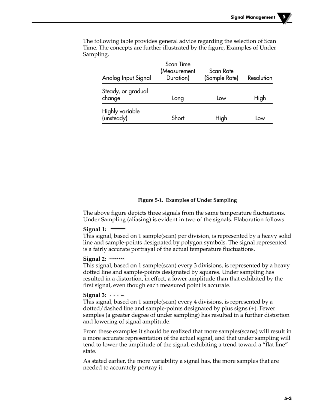
Figure 5-1. Examples of Under Sampling

The above figure depicts three signals from the same temperature fluctuations. Under Sampling (aliasing) is evident in two of the signals. Elaboration follows:

Signal 1:

This signal, based on 1 sample(scan) per division, is represented by a heavy solid line and sample-points designated by polygon symbols. The signal represented is a fairly accurate portrayal of the actual temperature fluctuations.

Signal 2:

This signal, based on 1 sample(scan) every 3 divisions, is represented by a heavy dotted line and sample-points designated by squares. Under sampling has resulted in a distortion, in effect, a lower amplitude than that exhibited by the first signal, even though each measured point is accurate.

Signal 3:

This signal, based on 1 sample(scan) every 4 divisions, is represented by a dotted/dashed line and sample-points designated by plus signs (+). Fewer samples (a greater degree of under sampling) has resulted in a further distortion and lowering of signal amplitude.

From these examples it should be realized that more samples(scans) will result in a more accurate representation of the actual signal, and that under sampling will tend to lower the amplitude of the signal, exhibiting a trend toward a “flat line” state.

As stated earlier, the more variability a signal has, the more samples that are needed to accurately portray it.

5-3