HP 35s Scientific L, E, P, Power, –139.0088, Example 2:, Logarithmic, Exponential, Statistics Programs, Prompts for hypothetical x–value

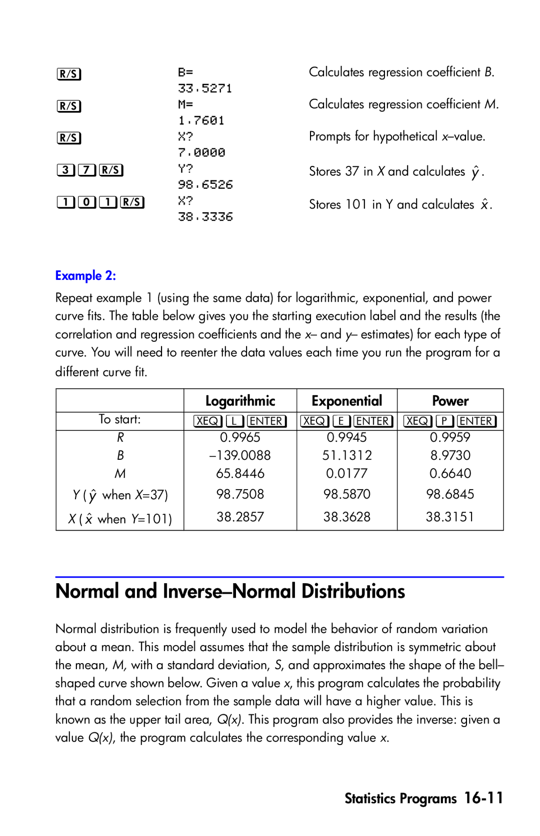
		Calculates regression coefficient B.
	
		Calculates regression coefficient M.
	
		Prompts for hypothetical x–value.
	
		Stores 37 in X and calculates yˆ.
	
		Stores 101 in Y and calculates xˆ.
	

Example 2:

Repeat example 1 (using the same data) for logarithmic, exponential, and power curve fits. The table below gives you the starting execution label and the results (the correlation and regression coefficients and the x– and y– estimates) for each type of curve. You will need to reenter the data values each time you run the program for a different curve fit.

	Logarithmic	Exponential	Power
To start:	L	E	P
R	0.9965	0.9945	0.9959
B	–139.0088	51.1312	8.9730
M	65.8446	0.0177	0.6640
Y ( yˆ when X=37)	98.7508	98.5870	98.6845
X ( xˆ when Y=101)	38.2857	38.3628	38.3151

Normal and Inverse–Normal Distributions

Normal distribution is frequently used to model the behavior of random variation about a mean. This model assumes that the sample distribution is symmetric about the mean, M, with a standard deviation, S, and approximates the shape of the bell– shaped curve shown below. Given a value x, this program calculates the probability that a random selection from the sample data will have a higher value. This is known as the upper tail area, Q(x). This program also provides the inverse: given a value Q(x), the program calculates the corresponding value x.

Statistics Programs 16-11