Manuals / Brands / Computer Equipment / Calculator / HP / Computer Equipment / Calculator

HP 35s Scientific Verifying the Result, value, value of y, Stores 11 in F and, calculates x and y, See appendix D for more information about how SOLVE works

1 382

Download 382 pages, 3.47 Mb

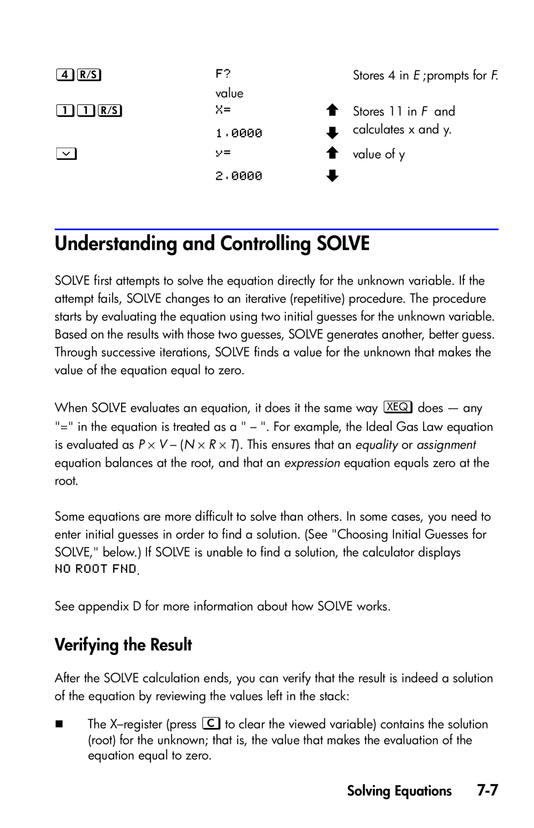
		Stores 4 in E ;prompts for F.
	value
		Stores 11 in F and
		calculates x and y.
Ø		value of y
	

Understanding and Controlling SOLVE

SOLVE first attempts to solve the equation directly for the unknown variable. If the attempt fails, SOLVE changes to an iterative (repetitive) procedure. The procedure starts by evaluating the equation using two initial guesses for the unknown variable. Based on the results with those two guesses, SOLVE generates another, better guess. Through successive iterations, SOLVE finds a value for the unknown that makes the value of the equation equal to zero.

When SOLVE evaluates an equation, it does it the same way does — any "=" in the equation is treated as a " – ". For example, the Ideal Gas Law equation is evaluated as P ⋅ V – (N ⋅ R ⋅ T). This ensures that an equality or assignment equation balances at the root, and that an expression equation equals zero at the root.

Some equations are more difficult to solve than others. In some cases, you need to enter initial guesses in order to find a solution. (See "Choosing Initial Guesses for SOLVE," below.) If SOLVE is unable to find a solution, the calculator displays

  .

See appendix D for more information about how SOLVE works.Verifying the Result

After the SOLVE calculation ends, you can verify that the result is indeed a solution of the equation by reviewing the values left in the stack:

The X–register (press to clear the viewed variable) contains the solution (root) for the unknown; that is, the value that makes the evaluation of the equation equal to zero.

Solving Equations 7-7

Contents

HP 35s scientific calculator REGISTER YOUR PRODUCT AT: www.register.hp.com Contents Complex number display format (, , ·‚) SHOWing Full 12–DigitPrecision Fractions Calculator Memory RPN: The Automatic Memory Stack Reusing Numbers with LAST X Chain Calculations in RPN Mode Work from the Parentheses Out Order of Calculation 4. Real–NumberFunctions Entering Fractions Display Rules Setting the Maximum Denominator Choosing a Fraction Format 6. Entering and Evaluating Equations 4Contents Operator Precedence Equation Functions Solving Equations For More Information Integrating Equations Operations with Complex Numbers 10.Vector Arithmetic 11.Base Conversions and Arithmetic and Logic Arithmetic in Bases 2, 8, and 16 The Representation of Numbers Negative Numbers Range of Numbers 13.Simple Programming Clearing One or More Programs The Checksum Nonprogrammable Functions Programming with BASE 14.Programming Techniques Branching (GTO) Loops Conditional Loops (GTO) Indirectly Addressing Variables and Labels 15.Solving and Integrating Programs 16.Statistics Programs Curve Fitting Normal and Inverse–NormalDistributions Grouped Standard Deviation B. User Memory and the Stack B-1 C. ALG: Summary D. More about Solving D-1 E. More about Integration E-1 E-2 Conditions That Prolong Calculation Time E-7 Page Basic Operation Page Getting Started Shifted Keys 1-2 Getting Started Alpha Keys Left-shiftedfunction Right-shifted Letter for alphabetic function Backspacing and Clearing Keys for Clearing Key Description Backspace Keys for Clearing (continued) The CLEAR menu (       ) indirect variables If you press (), a new menu     is displayed so you can verify your decision before erasing Using Menus HP 35s Menus Menu Chapter Name ÕÖ×Ø 3.Press while the item is underlined or  8 Exiting Menus 1-8 Getting Started Pressing RPN and ALG Modes To select RPN mode: 9{ 9{ ALG RPN mode Note 1-10 Getting Started Undo key The Display and Annunciators First Line Second Line The display comprises two lines and annunciators Annunciators HP 35s Annunciators Annunciator Meaning EQN RAD or GRAD HP 35s Annunciators (continued) the display of the entry in line 1 or line 2. Both of these annunciators may appear simultaneously, indicating that there are an entry. Entries in line 1 with missing Making Numbers Negative The key changes the sign of a number To key in a negative number, type the number, then press  In ALG mode, you may press key before or after typing the number mantissa z  1-16 Getting Started Understanding Entry Cursor Range of Numbers and OVERFLOW Single Argument or Unary Operations 1-18 Getting Started In RPN,RPN Program In ALG, Equation, ALG Program Two Argument or Binary Operations Õ 1-20 Getting Started In RPN, RPN Program x √ y XROOT(, ) 8 rounded Fixed–DecimalFormat () Scientific Format () Engineering Format () 1-22 Getting Started 8 Periods and Commas in Numbers () () 8( 8 Select full floating point precision (ALL format) 8( 8 separator 6 8  8 ) or 8× 8 Entering Fractions 1-26 Getting Started É   The decimal point is interpreted in the normal way Add ¾ to 12 3/8 Switch back to the current display mode Refer to chapter 5, "Fractions," for more information about using fractions Checking Available Memory 1-28 Getting Started Clearing All of Memory Page RPN: The Automatic Memory Stack 2-2 RPN: The Automatic Memory Stack The X and Y–Registersare in the Display Clearing the X–Register Reviewing the Stack the registers themselves maintain their positions, and only the X– and R (Roll Up) Exchanging the X– and Y–Registersin the Stack Press  The keystrokes to calculate this expression from left–to–right are:  2-4 RPN: The Automatic Memory Stack 1.The stack "drops" its contents. The T–(top)register replicates its contents 2.The stack "lifts" its contents. The T–register'scontents are lost 3.The stack drops former when the next number enters the How ENTER Works 4. Now enter and add two new numbers: 5+6 1 lost 2 lsot How to Clear the Stack writes 1.Press  2.Press  3.Press () (Mainly used during program entry.) 1.Lifts the stack 3.Overwrites the X–register 4.Clears x by overwriting it with zero 5.Overwrites x (replaces the zero.) Pressing returns this value into the X–register Correcting Mistakes with LAST WrongMistake: Correction: Calculation: Ù Reusing Numbers with LAST Calculate 96.704 + 52.3947 2-10 RPN: The Automatic Memory Stack Enters first number Intermediate result Final result To Rigel Centaurus: 4.3 yr ⋅ (9.5 ⋅ 1015 m/yr) To Sirius: 8.7 yr ⋅ (9.5 ⋅ 1015 m/yr) Work from the Parentheses Out Keys:Display:Description: 2-12 RPN: The Automatic Memory Stack Calculate 2 ⎟ (3 + 10): Calculates (3 + 10) first correct: 2 ⎟ Calculate 4 ⎟ [14 + (7 ⋅ 3) – 2] : Calculates (7 ⋅ 3) Exercises (16.3805x5) = 181.0000 Order of Calculation 2-14 RPN: The Automatic Memory Stack Page More Exercises 2-16 RPN: The Automatic Memory Stack Page Page Storing Data into Variables Enter the expression, then proceed as in the previous example different To store a copy of a displayed number (X–register)to a direct variable: Press letter–key  To recall a copy of a number from a direct variable to the display: A  “” prompts for variable Clears the number in the display The A..Z annunciator Turns on The VAR catalog 3-4 Storing Data into Variables Clear all direct variables C Store 3 in C, 4 in D, and 5 in E D E u()  Storage Arithmetic 3-6 Storing Data into Variables A Recall Arithmetic A  D D E F 3-8 Storing Data into Variables A Page Real–NumberFunctions To Calculate: Press: 4-2 Real–NumberFunctions Result: Entering π Setting the Angular Mode Option GRAD Trigonometric Functions 4-4 Real–NumberFunctions Page 4-6 Real–NumberFunctions Page CONST Menu Items Value 4-8 Real–NumberFunctions Page The HP 35s supports four types of conversions. You can convert between: rectangular and polar formats for complex numbers degrees, radians, and gradients for angle measures decimal and hexagesimal formats for time (and degree angles) Rectangular/Polar Conversions 4-10 Real–NumberFunctions 30o 8 8 6 4-12 Real–NumberFunctions Time Conversions To convert between decimal format and hours minutes, and seconds: 1.Enter the number you wish to convert 2.Press to convert to hours/degrees, minutes, and seconds or press 5to convert back to decimal format Unit Conversions To Convert: To: Displayed Results: 4-14 Real–NumberFunctions Factorial factorial *(the right–shifted key) Gamma gamma function Example: Combinations of People Twenty–fourpeople grouped six at a time Total number of combinations possible probability for that event x2 + y To calculate: Press:Display: 4-18 Real–NumberFunctions Fractions Display Rules 5-2 Fractions Entered Value Internal Value Displayed Fraction Accuracy Indicators You can set the maximum denominator that's used You can select one of three fraction formats The next few topics show how to change the fraction display Setting the Maximum Denominator The /c value defines only the maximum denominator used in Fraction–displaymode 5-4 Fractions Page Choosing a Fraction Format Most precise fractions Factors of denominator Fixed denominator. Fractions always use the /c value as the denominator Flag 7 toggles fraction-displaymode on or off; clear=off and set=on To Get This Fraction Format: Change These Flags: Examples of Fraction Displays How 2.77 Is Displayed /c Most Precise Factors of Denominator D 7/ inches Rounds the width to this value Width of six sections D 5-10 Fractions Entering and Evaluating Equations  D  6-2 Entering and Evaluating Equations equation list Operation Enters and leaves Equation mode Evaluates the displayed equation. If the equation is an assignment Variables in Equations ) and 6-4 Entering and Evaluating Equations Numbers in Equations Functions in Equations Parentheses in Equations   6-6 Entering and Evaluating Equations To display equations: To view a long equation: 14 characters long, only 14 characters are shown. The indicates more characters to the right 3.Press Öor Õto scroll the long equations in line 2 by a screen To edit an equation you're typing: 3.Press (or ) to save the equation in the equation list To edit a saved equation: Display the desired equation, press Using menus while editing an equation: Equalities Assignments Expressions 6-10 Entering and Evaluating Equations Type of Equation Result for  Result for  Using ENTER for Evaluation typing ends assignment If the equation is an equality or expression, the entire equation is evaluated Using XEQ for Evaluation 6-12 Entering and Evaluating Equations Responding to Equation Prompts To display digits hidden by the prompt, press  Equations follow certain conventions that determine how they're evaluated: How operators interact What functions are valid in equations Operator Precedence 6-14 Entering and Evaluating Equations Order Example Equations Equation Functions 6-16 Entering and Evaluating Equations RPN Operation Equation function sin cos(π /n) sin(π/n)  Õ Syntax Errors Example: Checksum and Length of an Equation 6-20 Entering and Evaluating Equations Solving Equations If the displayed value is the one you want, press  You can halt a running calculation by pressing or  Example: Solving the Equation of Linear Motion The equation of motion for a free–fallingobject is: d = v0 t + 1/2 g t G Displays the equation for for G for T P   the equation 7-4 Solving Equations P Solving built-inEquation 7-6 Solving Equations Stores 11 in F and calculates x and y value of y Verifying the Result approximation The Z– register (press Interrupting a SOLVE Calculation to view it without disturbing the stack, but solving cannot be resumed Choosing Initial Guesses for SOLVE The two initial guesses come from: The number currently stored in the unknown variable Entering your own guesses has the following advantages: d= v0 t + 1/2 gt y = t + log results in an error if x ≤ 0 (message   ) 40 40_2H 4 HÕ 7-10 Solving Equations 4 H   7-12 Solving Equations Integrating Equations I = ∫ab f (x) dx To integrate an equation: lower Display the equation: Press Select the variable of integration: Press variable 1 π J0 (x) = π ∫0 cos(x sin t)dt X sin sinx X  X approximates might Specifying Accuracy precision accuracy no more than in the integrand's values Example: Specifying Accuracy 8  () Displays the current Equation. The integral approximated to two decimal places The uncertainty of the approximation of the integral Example: Changing the Accuracy 8-8 Integrating Equations Operations with Complex Numbers 9-2 Operations with Complex Numbers Functions for One Complex Number, z Arithmetic With Two Complex Numbers, z1 and z2 8() 6 8() 6 6 6 6 6 6 imaginary real 185 lb 62 o 170 lb 143 o 100 lb261 o Sets Degrees mode Sets complex mode Evaluate 1i1+3θ 10+5θ 9() 8 θ Enters Enters 3θ Program lines: (ALG mode) 9-8 Operations with Complex Numbers Vector Arithmetic 3 3 Õ 3 10-2 Vector Arithmetic 9() 3  Calculate [-2,4]÷2 9() 3 Õ  3  Enters [3,4] Dot product 3 3 10-4 Vector Arithmetic Angle between vectors The angle between two vectors, A and B, can be found as θ θ ACOS(A B/ AB ) Find the angle between two vectors: A=[1,0],B=[0,1] 3   vector [0,5] Multiplies two vectors Divides two values 10-6 Vector Arithmetic Program lines: hand either (I) or (J) For example, to construct the vector [ C, REGZ, (J) ] in RPN mode, press d 3, then hC <Õ hA 10-8 Vector Arithmetic Base Conversions and Arithmetic and Logic an octal number. To enter an octal number, type the number followed by “” binary number. To enter a binary number, type the number followed by “” Examples: Converting the Base of a Number Õ  LOGIC Menu 11-4 Base Conversions and Arithmetic and Logic Here are some examples of arithmetic in Hexadecimal, Octal, and Binary modes: 12F16 + E9A16 77608 – 43268 Sets base 16; HEX annunciator on. Result Negative Numbers 11-6 Base Conversions and Arithmetic and Logic Range of Numbers Range of Numbers for Base Conversions Base Positive Integer Negative Integer Windows for Long Binary Numbers Using base in program and equations 11-8 Base Conversions and Arithmetic and Logic Statistical Operations Entering One–VariableData Entering Two–VariableData Correcting Errors in Data Entry 12-2 Statistical Operations To correct statistical data: Reenter the incorrect data, but instead of pressing 2.Enter the correct value(s) using  Initial x, y Corrected x, y s,σ Mean 12-4 Statistical Operations Page ÕÕ(  ) Four data pairs accumulated Calculates the mean price weighted for the quantity purchased Sample Standard Deviation Press () for the standard deviation of x–values Press Õ() for the standard deviation of y–values Example: Sample Standard Deviation Clears the statistics registers Population Standard Deviation ÕÕÕ Linear Regression L.R. (Linear Regression) Menu Menu Key  ˆ Õ ˆ 12-8 Statistical Operations (70, y) r m b Õ( ˆ ) Enters hypothetical x–value The predicted yield in tons per hectare Normalizing Close, Large Numbers Effect of Deleted Data Summation Statistics Pressing gives you access to the contents of the statistics registers: () to recall the number of accumulated data sets Press Õ() to recall the sum of the x–values Press ÕÕ() to recall the sum of the y–values Access to the Statistics Registers Statistics Registers Register Number 12-12 Statistical Operations 7  7 Page Programming Page Simple Programming 13-2 Simple Programming Keys:Display: (In ALG mode) X  Selecting a Mode Program Boundaries (LBL and RTN) return Notice that the line numbers acquire an  to match their label Program Labels routines Data Input and Output These are covered later in this chapter under "Entering and Displaying Data To enter a program into memory: 1.Press to activate Program–entrymode program pointer Give the program a Clear functions and backspace key Function Names in Programs A 13-8 Simple Programming E R R PRGM Executing a Program (XEQ) Press label to execute the program labeled with that letter: If necessary, enter the data before executing the program A   E  Testing a Program Value of π 25π In a program, you can get data in these ways: From variables that already have values stored In a program, you can display information in these ways: Using INPUT for Entering Data Variable where "R" is the variable's name "?" is the prompt for information, and To respond to a prompt: 13-14 Simple Programming Using VIEW for Displaying Data display only Pressing copies this number to the X–register Pressing (or ) erases the VIEW display and shows the X–register Pressing clears the contents of the displayed variable Using Equations to Display Messages  ÇR ÇH 13-16 Simple Programming  R H V  R 4R H  V OL  A RE A V Displaying Information without Stopping 13-18 Simple Programming Programming a Stop or Pause (STOP, PSE) Interrupting a Running Program Error Stops To delete a program line: Select the relevant program or routine and press 3.Key in the new instruction, if any. This replaces the one you deleted 4.Exit program entry ( or ) To insert a program line: Viewing Program Memory Press to move the program pointer to   Press label nnn to move to a specific line Memory Usage The Catalog of Programs (MEM) Execute a labeled program. (Press or while the label is displayed.) Display a labeled program. (Press while the label is displayed.) Delete specific programs. (Press while the label is displayed.) Clearing One or More Programs The Checksum 67 bytes The following functions of the HP 35s are not programmable: label line number Ø, × 13-24 Simple Programming Selecting a Base Mode in a Program Numbers Entered in Program Lines Decimal mode set: Ax4 + Bx3 + Cx2 + Dx + E Write a program using RPN operations for 5x4 + 2x3, then evaluate it for x 13-26 Simple Programming A X A  13-28 Simple Programming Programming Techniques A subroutine can itself call other subroutines The flow diagrams in this chapter use this notation:    line number marked  1 ("from 1") Nested Subroutines 14-2 Programming Techniques Page 14-4 Programming Techniques A Programmed GTO Instruction Using GTO from the Keyboard 14-6 Programming Techniques Tests of Comparison (x?y, x?0) The Test Menus Program Lines: 14-8 Programming Techniques Flags Meanings of Flags overflow automatically Flag Fraction–ControlFlags Clear 14-10 Programming Techniques Flag 10 controls program execution of equations: 1.Program execution halts 2.The program pointer moves to the next program line it doesn't affect automatic prompting during keyboard execution Flag 11 is automatically cleared after evaluation, SOLVE, or Annunciators for Set Flags Using Flags Pressing displays the FLAGS menu:    FLAGS Menu  n Page Use above program to see how to use flags S  value   value Executes label S; prompts for X value Stores 1 in X; prompts Y value Begins the fraction program Clears three fraction flags Displays messages Selects decimal base Prompts for a number F Executes label F; prompts for a fractional number (V) Stores 2.53 in V; prompts for denominator (D) little below shows the fraction Conditional Loops (GTO) Loops with Counters (DSE, ISG) When you want to execute a loop a specific number of times, use the  ) or For a count–downloop, use variable For a count–uploop, use variable ccccccc fffii ccccccc — fff fff The Variables "I" and "J 14-20 Programming Techniques STO INPUT DSE The Indirect Address, (I) and (J) I to J If I/J contains: Then (I)/(J) will address: variable A or label A variable Z or label Z error: Program Control with (I)/(J) index Equations with (I)/(J) ) or (J) indirect “12345” into address storage range is now “0-150” still “0-150” Display “INVALID (I)”, because address “170” is undefined Solving and Integrating Programs Begin the program with a unknown separate every 3.Enter the instructions to evaluate the function G H P V N R L H  P   L  Selects variable P; prompts for 15-6 Solving and Integrating Programs Program Lines: (In RPN mode) Checksum and length: 62A0 11         Checksum and length: D45B 18    Setup for Index for 15-8 Solving and Integrating Programs Si(t) = ∫ t )dx ∫ M dD Q(D) 15-10 Solving and Integrating Programs Recalls lower limit of integration Recalls upper limit of integration. (X = D.) Specifies the function Integrates the normal function using the dummy variable D Page Statistics Programs y = BeMx y = B + Mx y = BxM y = B + MIn Page 16-4 Statistics Programs Page Checksum and length: 889C Calculates xˆ = e(Y – B) ⎟ M Checksum and length: 0DBE Calculates yˆ= BeMX Branches to M005 Page Flags Used: Program instructions: 1.Key in the program routines; press when done 2.Press and select the type of curve you wish to fit by pressing: Sfor a straight line; S  16-10 Statistics Programs Prompts for hypothetical x–value Stores 37 in X and calculates yˆ Example 2: Logarithmic L E P –139.0088 "Upper tail" area Q(x) = 0.5 − σ 12π ∫xx e−((x −x )⎟σ )2 ⎟2dx 16-12 Statistics Programs Page 16-14 Statistics Programs Page 5.To calculate X given Q(X), skip to step 9 of these instructions 6.To calculate Q(X) given X, D 9.To calculate X given Q(X), press I After the prompt, key in the value of S  16-16 Statistics Programs D  S   Starts the initialization routine Stores 55 for the mean Enters 90 for X and calculates Q(X) I   Page 16-20 Statistics Programs Page Group U  16-22 Statistics Programs G  Page Miscellaneous Programs and Equations P 4 4 I NÕ I loan Part Keys:Display: (In RPN mode) 17-4 Miscellaneous Programs and Equations Page I 17-6 Miscellaneous Programs and Equations Page 17-8 Miscellaneous Programs and Equations Page 17-10 Miscellaneous Programs and Equations v2=U i + V j + W k 17-12 Miscellaneous Programs and Equations z Page Appendixes and Reference Page Support, Batteries, and Service A-2 Support, Batteries, and Service A-2 The calculator is powered by two 3-voltlithium coin batteries, CR2032 To install batteries: Have two fresh 用 BK+B A-3 A-4 Support, Batteries, and Service A-4 Reset Hole If these steps fail to restore calculator operation, it requires service Do the 3.Contact the Calculator Support Department listed on page A–8 A-5 A-6 Support, Batteries, and Service A-6 HP 35s Scientific Calculator; Warranty period: 12 months HP warrants to you, the Support, Batteries, and Service A-7 A-7 Country : Telephone numbers Australia 1300-551-664or A-8 Support, Batteries, and Service A-9 A-9 A-10 Support, Batteries, and Service A-10 Support, Batteries, and Service A-11 A-11 •Reorient or relocate the receiving antenna •Increase the separation between the equipment and the receiver •Consult the dealer or an experienced radio or television technician for help Modifications A-12 Houston, TX 77269-2000or call HP at Canadian Notice Avis Canadien European Union Regulatory Notice A-13 Japanese Notice VCCI Perchlorate Material - special handling may apply A-14 Support, Batteries, and Service A-14 User Memory and the Stack To see the memory requirements of specific equations in the equation list: If necessary, scroll through the equation list (press To see the total memory requirements of specific programs: 1.Press () to display the first label in the program list B-2 1.Press and hold down the key 2.Press and hold down ¥ User Memory and the Stack B-3 B-3 Category CLEAR ALL MEMORY CLEAR (Default) B-4 Disabling Operations Neutral Operations User Memory and the Stack B-5 B-5 ˆ ˆ B-6 User Memory and the Stack B-7 B-7 B-8 ALG: Summary 5.Unary Minus + 6.⋅, ⎟ 7.+, – 8 Simple Arithmetic Here are some examples of simple arithmetic To Calculate:Press:Display: 12 + 12 – Power Functions Õ64 Percentage Calculations Õ27 Õ12 Permutations and Combinations xÕ Total number of Quotient and Remainder Of Division (⎟)Integer 1 ÕInteger 2. 4  No calculation is done Õ  Calculates 85 − Hyperbolic functions C-6 ALG: Summary C-6 ALG: Summary C-7 C-7 To enter a complex number: C-8 ALG: Summary C-8 6 ALG: Summary C-9 C-9 8Ë Õ4 66 4 6Õ4 6 F E9A A0 ALG: Summary C-11 C-11 6 {Ž Z z C-12 ALG: Summary C-12   ˆ Õ ˆ ALG: Summary C-13 C-13 C-14 More about Solving f (x) Function Whose Roots Can Be Found D-2 More about Solving D-2 If it finds an estimate for which f(x) equals zero. (See figure a, below.) Example: An Equation With One Root Find the root of the equation: –2x3 + 4x2 – 6x + 8 D-3 Select Equation mode Enters the equation X X X Now, solve the equation to find the root: X _  X X X D-5 Special Case: A Discontinuity and a Pole XÕ D-6 More about Solving D-6 X _  − 1 X4 Õ More about Solving D-7 X _  D-8 More about Solving D-8 Case Where No Root Is Found D-9 X    X  D-10 More about Solving D-10 X4 X ÕÕ D-11 X   D-12 X _  More about Solving D-13 D-13 D-14 More about Integration whose E-2 More about Integration E-2 For example, consider the approximation of ∫0∞ xe−xdx E-3   E-4 E-5 E-6 More about Integration E-6 Rerun the previous integration problem with this new limit of integration:   New upper limit X  ∫   Integral. (The calculation takes a minute or two.) Uncertainty of approximation E-8 E-9 E-10 Messages F-2 Messages F-2 Messages F-3 F-3 SOLVE (include EQN and PGM mode)cannot find the not found, point of interest, left unequal to right. A SOLVE operation executed in a program does not to skip the next program line (the line following the F-4 Statistics error: Attempted to do a statistics calculation with n Attempted to calculate sx sy, xˆ , yˆ , m, r, or b with n Attempted to calculate r, xˆ or xw with x–dataonly (all y–valuesequal to zero) F-5 F-6 Operation Index ÖorÕ Ø G-2 Operation Index G-2 ÕÕÕÕÕ ÕÕÕÕ ∑(xi − x)2 ⎟ n ÕÕÕ(σ) ∑(yi − y)2 ⎟ n ÕÕÕÕ() G-4 Operation Index G-4 BIN CF n G-5 G-6 Operation Index G-6 G-7 (I)/(J) 7/A G-8 Operation Index G-8 Operation Index G-9 G-9 ÕÕÕ() G-10 Operation Index G-10 ∑(xi − x)(yi − y) G-12 Operation Index G-12 G-13 ∑(xi − x)2 ⎟ (n − 1) ∑(yi − y)2 ⎟ (n − 1) G-14 Operation Index G-14 ÕÕ Õ(≤) ÕÕÕ(>) ÕÕÕÕ(≥) Operation Index G-15 Õ ≤ ÕÕÕ(>) ÕÕÕÕ(≥) ÕÕÕÕÕ(=) 8 G-17 G-18 Index Index-2 Index-3 memory in 13-16multiple roots 7-9no root 7-8numbers in numeric value of 6-10, 6-11, 7-1, 7-7 15-1, 15-8roots scrolling 6-7, 13-7, 13-16solving 7-1, D-1 stack usage finds PRGM TOP 13-6, 13-21,14 finds program labels 13-10,13- 22 finds program lines 13-22, 14-5gamma function go to. See GTO grads (angle units) 4-4, A-2Grandma Hinkle 12-7Greatest integer logarithmic functions 4-1, 9-3, C-5logic loop counter 14-18, 14-23looping 14-16, 14-17Łukasiewicz program catalog 1-28, 13-22reviews memory 1-28variable catalog mantissa mass conversions 4-14math periods and commas in 1-23, A-1precision D-13 prime Ä1-1 one-variablestatistics 12-2overflow flags 14-9, F-4 Index-8 rolling the stack 2-3, C-7root functions 4-3roots. See SOLVE checking 7-7, D-3in programs 15-6multiple none found 7-8, D-8of equations 7-1of programs rounding fractions 5-8, 13-18numbers Index-10 angle between two vectors Index-11