Sprint Service
Intellectual Property Notices
Page
Page
Table of Contents
Your Sprint Power VisionSM and Other Wireless Connections
205
3C. Using Messaging
225
211
317
293
307
Your Resources
Index
Page
Welcome and thank you for choosing Sprint
Welcome to Sprint
How to Use This Guide
While Using Your Treo
Where to Learn More
For a Quick Introduction
If You Need More Information
Sprint
Managing Your Account
From the Today Screen on Your Treo
From Any Other Phone
Sprint Operator Services
Page
Your Setup
Page
Setting Up Your Palm Treo 800W Smart Device
Setting Up Your Palm Treo 800W SmartDevice
What You Need
Experience SprintSpeed Basics Guide Set Up Your Email
Hardware
Documentation
Tip
Software
Front View
Your Treo Smart Device
Device Setup
Back View
Device Setup
Inserting the Battery
Charging the Battery
Checking Battery Power
Maximizing Battery Life
Did you know?
Setting Up Service
Setting Up Service
Waking Up the Screen and Turning It Off
Power/End Phone/Talk Center Start Calendar Inbox
Turning Your Palm Treo 800W SmartDevice On and Off
Turning Your Phone On and Off
Before You Begin
Making Your First Call
What’s My Phone Number?
Adjusting Call Volume
Select Preferences Phone Settings
To set up your voicemail
Setting Up Your Voicemail
Sprint Power VisionSM Password
Creating Sprint Account Passwords
Account Password Voicemail Password
Connecting to Your Computer
Connecting to Your Computer
Synchronizing With Desktop Sync Software
Synchronization Methods
What Can I Synchronize?
Synchronizing Wirelessly With the Server
Did you know?
Computer
System Requirements
Setting Up Your Computer for Synchronization
Installing ActiveSync Desktop Software Windows XP
Setting Up Windows Mobile Device Center Windows Vista
Using the Desktop Sync Software
ActiveSync window
Synchronizing With a USB Connection
Connect the sync cable to the bottom of your Treo
Tip
Your Palm Treo 800W Smart Device
Page
Moving Around on Your Palm Treo 800W Smart Device
Moving Around on Your Palm Treo 800W SmartDevice
Moving Around on the Screen
Scrolling Through Screens
Highlighting and Selecting Items
Closing Screens
Highlighting Text
Using the Softkeys
Selecting Menu Items
Selecting Items in a Shortcut Menu
Selecting Options in a List
Understanding the Backlight
Using the Keyboard
Entering Lowercase and Uppercase Letters
Entering Other Symbols and Accented Characters
Entering Numbers, Punctuation, and Symbols
Entering Passwords
Tip
Then press… To select… Ä â ã å æ
Symbols and Accented Characters
Or B † ‡ † ‡ Ð Ë ê
Or L Ö ô œ õ
+ E ¼ ½ + R + T + J + H € £ ¥ ¢ + K + N
Then press… To select… Ü û
Opening and Closing Applications
Using the Buttons
Using the Start Menu
Closing Applications
Using Your Today Screen
Did you know?
Moving Around on Your Palm Treo 800W Smart Device
Using the Phone Features
Using the Phone Features
Dialing With the Keyboard
Accessing Your Today Screen
Making Calls
Dialing by Contact Name
Dialing With a Speed-Dial Button
Dialing From a Web Page or Message
Dialing by Company Name
Redialing a Recently Called Number
Press Phone/Talk
Dialing Using the Onscreen DialPad
Receiving Calls
Press Power/End
Setting Up Voicemail
Using Voicemail
Retrieving Voicemail From a Notification
Retrieving Voicemail Messages From the Today Screen
Tip
Select Clear Voicemail Icon and then press Center
What Can I Do When I’m On a Call?
Clearing the Voicemail Icon
Returning to a Call From Another Application
Saving Phone Numbers
Ending a Call
Forwarding Calls
Managing Multiple Calls
Making a Second Call
Answering a Second Call Call Waiting
Making a Conference Call
Using Flash Mode During a Call
Select Send Key Flash to enter Flash mode
Setting Up and Managing Speed-Dial Buttons
Creating a Speed-Dial Button
Systems
Arranging Your Speed-Dial Buttons
Editing a Speed-Dial Button
Deleting a Speed-Dial Button
You can connect a phone headset for hands-free operation
Using a Phone Headset
Using the Phone Features
Using a Hands-Free Device With Bluetooth Wireless Technology
Headset Specifications
Before You Begin
On the Personal tab, select Sounds & Notifications
Customizing Phone Settings
Selecting Ringtones and Vibrate Settings
100
Adjusting Volume Settings
Assigning a Picture and Ringtone ID to a Contact
Selecting Your Call Settings
Using the Phone Features 101
102
Setting Your Dialing Preferences
Using the Phone Features 103
Setting Your Abbreviated Dialing Preferences
Selecting Your Privacy Settings
Selecting Your Data Settings
Select the Services tab and Location Privacy
104
Controlling Your Roaming Experience
Selecting Your HAC Settings
Using the Phone Features 105
106
Feature Availability
Setting Roaming Preferences
Using the Phone Features 107
Checking Signal Strength and Phone Status
108
Using the Phone Features 109
110
Your Sprint Power VisionSM and Other Wireless Connections
112
Sprint Power VisionSM-The Basics 113
Sprint Power VisionSM-The Basics
Enabling Sprint Power Vision
Getting Started With Sprint Power Vision
Sprint Power Vision Username
Accessing Sprint Power Vision
Sprint Power Vision Symbols on Your Screen
Sprint Power Vision Billing Information
To set up a USB Internet Sharing connection
Using Your Palm Treo 800W SmartDevice as a Modem
Setting Up an Internet Connection With Your Computer
Sprint Power VisionSM-The Basics 117
118
Sprint Power VisionSM-The Basics 119
Using Sprint TV
To access your Sprint TV channels
Initializing Your Pocket Express Service
Using Pocket Express
Accessing Pocket Express Information
Select Get Pocket Express
Sprint Power VisionSM-The Basics 121
To automatically retrieve updates
To manually retrieve updates
Updating Pocket Express Information
Set the Frequency and Begin Time
Using the Email Features 123
Using the Email Features
Getting Started With Email
Microsoft Direct Push Technology
Using the Email Features 125
126
Setting Up an Exchange Server Account
Select ActiveSync
Using the Email Features 127
128
Using the Email Features 129
Setting a Sync Schedule With an Exchange Server
Setting Up Inbox to Work With Common Providers
Setting Up an Imap or POP Email Account
Select Setup E-mail
130
Using the Email Features 131
Setting Up Inbox to Work With Other Providers
Using the Email Features 133
134
Outgoing Smtp mail server Enter the server name
Using the Email Features 135
Selecting Which Email Account to Use
Sending and Receiving Email Messages
Creating and Sending an Email Message
136
Select Spell Check
Using the Email Features 137
138
Receiving Email Messages
Receiving Attachments
Using the Email Features 139
140
Downloading Attachments Automatically
Check the Include file attachments box
Working With Email Messages
Using the Email Features 141
Adding a Contact From an Email Message
Adding an Online Address Book
142
Using an Online Address Book
Finding Messages
Using the Email Features 143
144
Using Links in Messages
Replying to a Message
Using the Email Features 145
Using Inbox Shortcuts
Forwarding a Message
Deleting Messages
146
Adding a Signature to Your Messages
Using the Email Features 147
Customizing Your Inbox Settings
148
Using the Email Features 149
Changing Email Download Settings
Tip
Using the Email Features 151
Setting Email Delivery Preferences
152
Working With Meeting Invitations
Sending Email Messages From Within Another Application
Using the Email Features 153
154
Using Messaging 155
Using Messaging
156
About Messaging
Creating and Sending a Text Message
Using Messaging 157
Sending and Receiving Messages
Select Message Options 158
Setting Message Options
Receiving Text Messages
Using Messaging 159
160
Using Messaging to Chat
Viewing a Message
Message Status Icons
Using Messaging 161
Managing Your Messages
Deleting a Single Message
Sorting Your Messages
Deleting Multiple Messages
Select By Date or By Name
Using Messaging 163
Customizing Your Messaging Settings
Using Live Search for Windows Mobile
Using Windows LiveTM
Select Live Search
164
Select Windows Live Select Sign in to Windows Live
Setting Up Windows Live Mail
Using Messaging 165
166
Using Windows Live Messenger
Using Windows Live Mail
Using Messaging 167
Select Windows Live
Tip
Using Messaging 169
170
Browsing the Web 171
Browsing the Web
Press Start and select Internet Explorer
Viewing a Web
Browsing the Web 173
Press OK to close Internet Explorer Mobile
Working With Favorites
Viewing a Favorite
Creating a Favorite
Organizing Your Favorites
Select New Folder
Copying Text From a Web
Working With Web Pages
Downloading Files and Images From a Web
Browsing the Web 177
Customizing Your Internet Explorer Mobile Settings
Using the History List
Select the Memory tab and set any of the following options
Browsing the Web 179
Searching the Web From Your Today Screen
180
181
Using GPS
Using GPS
182
Finding a Point of Interest
Finding a Point of Interest Near Your Current Location
Finding a Point of Interest Near Another Location
Using GPS 183
184
Using Maps
Select the Map your current location link
Select Sprint Navigation
Using Sprint Navigation
Using GPS 185
186
Using Wireless Connections 187
Using Wireless Connections
Why Use a Wi-Fi Connection?
Connecting to a Wi-Fi Network
Are there different types of Wi-Fi networks?
188
Using Wireless Connections 189
Turning the Wi-Fi Feature On and Off
190
Wi-Fi Status Icons
Connecting to an Open Network
Using Wireless Connections 191
Connecting to a Secure Network
192
Using Wireless Connections 193
194
Disconnecting From a Wi-Fi Network
Customizing Wi-Fi Settings
Using Wireless Connections 195
Bluetooth status icon
Connecting to Devices With Bluetooth WirelessTechnology
Setting Up a Bluetooth Connection
196
Using Wireless Connections 197
198
Sending Information Over a Bluetooth Connection
Using Wireless Connections 199
Receiving Information Over a Bluetooth Connection
Synchronizing Over a Bluetooth Connection
200
Beaming Information With IR
Beaming a Record
Using Wireless Connections 201
202
Receiving Beamed Information
Synchronizing Over an Infrared Connection
Your Portable Media Device
204
Synchronizing Your Media Files 205
Synchronizing Your Media Files
206
Synchronizing Your Pictures, Videos, and Music
Synchronizing Pictures, Videos, and Music Windows XP
Synchronizing Your Media Files 207
208
Synchronizing Pictures, Videos, and Music Windows Vista
Synchronizing Your Media Files 209
210
Working With Your Pictures and Videos 211
Working With Your Pictures and Videos
Taking Pictures and Videos
About Your Camera
Taking a Picture
Press Start and select Pictures & Videos
Working With Your Pictures and Videos 213
Recording a Video
Taking Pictures in Burst Mode
Working With Your Pictures and Videos 215
Viewing a Picture
Viewing Pictures and Videos
Viewing a Video
216
Working With Your Pictures and Videos 217
Viewing a Slide Show
218
Sending Pictures and Videos
Organizing Pictures and Videos
Working With Your Pictures and Videos 219
Using a Picture as the Today Screen Background
220
Adding a Picture to a Contact Entry
Editing Pictures
Working With Your Pictures and Videos 221
Deleting a Picture or Video
Renaming a Picture or Video
222
Customizing Your Pictures & Videos Settings
Working With Your Pictures and Videos 223
224
Playing Media Files 225
Playing Media Files
226
AAC AMR QCP
Playing Media Files 227
Synchronizing Windows Media Player Library Files
228
Playing Media Files 229
Playing Media Files
230
Playing Media Files 231
Working With Libraries
Working With Playlists
Playing Media Files 233
Customizing Windows Media Player Mobile
234
Your Wireless Organizer
236
Using the Organizer Features 237
Using the Organizer Features
238
Contacts
Adding a Contact
Select Open Contact
Using the Organizer Features 239
Viewing or Changing Contact Information
240
Viewing a Map of a Contact’s Address
Deleting a Contact
Using the Organizer Features 241
Customizing Contacts
Finding a Contact in an Online Address Book
Displaying Your Calendar
Calendar
Press Calendar
242
Creating an Appointment
Using the Organizer Features 243
244
Creating an Untimed Event
Scheduling a Repeating Appointment
Using the Organizer Features 245
Adding an Alarm Reminder to an Event
246
Sending a Meeting Request
Select Attendees and then select Add Required Attendee
Marking an Event as Sensitive
Using the Organizer Features 247
Deleting an Event
Organizing Your Schedule
Customizing Calendar
248
Using the Organizer Features 249
250
Tasks
Adding a Task
Organizing Your Tasks
Checking Off a Task
252
Deleting a Task
Customizing Tasks
Recording a Voice Note
Using the Organizer Features 253
Creating a Note
254
Creating a Note From a Template
Organizing Your Notes
Using the Organizer Features 255
Deleting a Note
Customizing Notes
Select Calculator 256
Calculator
Performing Calculations
Using the Organizer Features 257
Using the Calculator Memory
258
Increasing Your Productivity 259
Increasing Your Productivity
260
Synchronizing Microsoft Office and Other Files
Synchronizing Files Windows XP
Increasing Your Productivity 261
262
Where Are the Changes I Made to My File?
Synchronizing Files Windows Vista
Increasing Your Productivity 263
Word Mobile
264
Opening an Existing Document
Creating a Document
Creating a Document From a Template
Select Word Mobile
266
Finding or Replacing Text in a Document
Moving orCopying Text
Formatting Text
Saving a Copy of a Document
Formatting Paragraphs and Lists
Increasing Your Productivity 267
268
Checking Spelling in a Document
Increasing Your Productivity 269
Organizing Your Documents
Deleting a Document
270
PowerPoint Mobile
Customizing Word Mobile
Playing a Presentation
Setting Presentation Playback Options
Select PowerPoint Mobile
272
Excel Mobile
Increasing Your Productivity 273
Select Excel Mobile
Creating a Workbook
Increasing Your Productivity 275
Creating a Workbook From a Template
276
Viewing a Workbook
Entering a Formula
Calculating a Sum
Inserting a Function
Increasing Your Productivity 277
278
Entering a Sequence Automatically
Adding Cells, Rows, and Columns
Increasing Your Productivity 279
Formatting Cells
Renaming a Worksheet
Formatting Rows and Columns
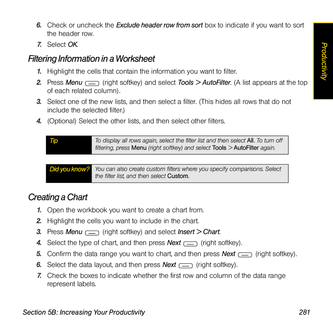
Sorting Information in a Worksheet
280
Increasing Your Productivity 281
Creating a Chart
Filtering Information in a Worksheet
282
Formatting or Changing a Chart
Finding or Replacing Information in a Workbook
Increasing Your Productivity 283
Organizing Your Workbooks
Deleting Cells, Rows, and Columns
284
Customizing Excel Mobile
Creating a New Note
OneNote Mobile
Select OneNote Mobile
Increasing Your Productivity 285
286
Viewing or Editing an Existing Note
Increasing Your Productivity 287
Renaming a Note
Sorting your Notes
288
Opening a File
Increasing Your Productivity 289
Customizing the Display
290
Your Information and Settings
292
Managing Files and Applications 293
Managing Files and Applications
294
Using Search
Finding Information
Managing Files and Applications 295
Exploring Files and Folders
296
Installing Applications
Click Bonus Software
Installing Bonus Software From the CD
Select Software Store
Managing Files and Applications 297
298
Installing Applications From Your Computer
Managing Files and Applications 299
Installing Applications Onto an Expansion Card
Getting Help With Third-Party Applications
300
Removing Applications
Sharing Information
Managing Files and Applications 301
Using Expansion Cards
302
Inserting and Removing Expansion Cards
Opening Applications on an Expansion Card
Managing Files and Applications 303
Saving Files to an Expansion Card
304
Moving Information Between Your Treo and anExpansionCard
Viewing Available Expansion Card Memory
Managing Files and Applications 305
Exploring Files on an Expansion Card
Renaming Files on an Expansion Card
306
Encrypting an Expansion Card
Check the Encrypt files placed on storage cards box
Synchronizing Information 307
Synchronizing Information
308
Setting Up Wireless Synchronization
Synchronizing Information 309
310
Setting the Synchronization Schedule
Synchronizing Information 311
Initiating a Wireless Sync Manually
312
Other Ways to Synchronize
Synchronizing Information 313
Synchronizing With Multiple Computers
Changing Which Applications Sync
Synchronizing Information 315
Stopping Synchronization
316
Customizing Your Palm Treo 800W Smart Device 317
Customizing Your Palm Treo 800W SmartDevice
Selecting Your Today Screen Background
Today Screen Settings
Changing the System Color Scheme
318
Customizing Your Palm Treo 800W Smart Device 319
System Sound Settings
Selecting Which Items Appear on Your TodayScreen
On the Personal tab, select Sounds & Notifications 320
Setting the Ringer Switch
Selecting Sounds & Notifications
Customizing Your Palm Treo 800W Smart Device 321
Adjusting the Brightness
Display and Appearance Settings
Changing the Text Size
322
Setting Display Formats
Aligning the Screen to Correct Tapping Problems
On the Alignment tab, select Align Screen
Customizing Your Palm Treo 800W Smart Device 323
Arranging the Start Menu
Application Settings
Reassigning Buttons
324
Using Voice Commands
Setting Up Voice Commands
On the Personal tab, select Voice Command
Customizing Your Palm Treo 800W Smart Device 325
326
Setting Input Options
Customizing Your Palm Treo 800W Smart Device 327
328
Locking Your Treo and Information
Customizing Your Palm Treo 800W Smart Device 329
Using Keyguard
Using Auto-Keyguard and TouchscreenLockout
330
Using Phone Lock
Customizing Your Palm Treo 800W Smart Device 331
Using System Password Lock
332
Entering Owner Information
Setting the Date and Time
System Settings
On the Personal tab, select Owner Information
Customizing Your Palm Treo 800W Smart Device 333
334
Synchronizing the Date, Time, and Time Zone With the Network
Customizing Your Palm Treo 800W Smart Device 335
Setting System Alarms
Managing Identity Certificates
336
Enabling Error Reporting
Customizing Your Palm Treo 800W Smart Device 337
Setting Up an External GPS Device
338
Viewing and Optimizing Power Settings
Viewing Memory Usage
Customizing Your Palm Treo 800W Smart Device 339
Viewing and Managing Active Tasks
340
Connection Settings
Turning Wireless Services On and Off
Connecting to a VPN
Managing ISP Settings
On the Tasks tab, select Manage existing connections
Customizing Your Palm Treo 800W Smart Device 341
On the Tasks tab, select Add a new VPN server connection
Setting Up a Proxy Server
On the Tasks tab, select Set up my proxy server 342
Customizing Your Palm Treo 800W Smart Device 343
Ending a Data Connection
Enrolling a Domain
344
Purchasing Accessories for Your Treo
Your Resources
346
Help 347
Help
348
Transferring Information From Another Device
Help 349
Resetting Your Palm Treo 800W SmartDevice
Performing a Soft Reset
350
Performing a Hard Reset
Help 351
Replacing the Battery
352
Help 353
Performance
Applications Are Running Slower Than Usual
Can’t Charge the Battery
Can’t Save or Access Files on an Expansion Card
Check the Receive all incoming beams box
354
Help 355
Screen
Screen Appears Blank
My Treo Won’t Connect to the Wireless Network
Signal Strength Is Weak
Network Connection
My Treo Seems to Turn Off by Itself
Help 357
Can’t Tell If Data Services Are Available
My Treo Won’t Connect to the Internet
358
Turn on Bluetooth box is checked in Bluetooth Settings
Can’t Send or Receive Text Messages
Help 359
On the Devices tab, select Add New Device
Desktop Sync Software
Synchronization
Desktop Sync Software Does Not Respond to a Sync Attempt
360
Help 361
362
Help 363
My Windows Media Player Library Won’t Sync
Synchronization Starts But Doesn’t Finish
My Appointments Show Up in the Wrong TimeSlotAfterI Sync
364
Help 365
Can’t Synchronize Using a Bluetooth Connection
Check the Use above setting when roaming box
Exchange ActiveSync wireless synchronization
Can’t Synchronize With My Company’s Exchange Server
My Scheduled Sync Doesn’t Work
Help 367
My Today Screen Settings Are Not Restored AfteraHardReset
An Alert Tells Me That the Server Could Not Be Reached
368
Have Problems Using My Account
Have Problems Sending and Receiving Email
Help 369
Have Problems Sending Email
Auto Sync Is Not Working
Web
Can’t Access a
My vCard or vCal Email Attachment Isn’t ForwardingCorrectly
370
An Image or Map Is Too Small on My TreoScreen
Camera
Secure Site Refuses to Permit a Transaction
Help 371
372
My Camera Won’t Take Pictures
Camera Preview Image Looks Strange
Help 373
Third-Party Applications
Getting More Help
Making Room on Your Treo
Is the Other Person Hearing an Echo?
Voice Quality
Are You Hearing Your Own Voice Echo?
Is Your Voice Too Quiet on the Other End?
376
Glossary 377
Glossary
378
Glossary 379
380
Your Safety and Specifications
382
Important Safety Information 383
Important Safety Information
384 Important Safety Information
General Precautions
Following Safety Guidelines
Using Your Phone While Driving
Using Your Treo Near Other Electronic Devices
Important Safety Information 385
386 Important Safety Information
Restricting Children’s Access to Your Treo
Turning Off Your Phone Before Flying
Turning Off Your Phone in Dangerous Areas
Box. Your Treo 800 W smart device phone has an M4/T4 rating
Using Your Phone With a Hearing Aid Device
Important Safety Information 387
Protecting Your Battery
Caring for the Battery
388 Important Safety Information
Getting the Best Hearing Device Experience With Your Treo
Important Safety Information 389
390 Important Safety Information
Knowing Radio Frequency Safety
Radio Frequency RF Energy
Disposal of Lithium-Ion Li-Ion Batteries
Body-Worn Operation
Specific Absorption Rate SAR for Wireless Phones
Important Safety Information 391
Description of ESD
Static Electricity, ESD, and Your Treo
FCC Radio Frequency Emission
Important Safety Information 393
Precautions Against ESD
ESD-Susceptible Equipment
Conditions That Enhance ESD Occurrences
Owner’s Record
394 Important Safety Information
User Guide Proprietary Notice
Serial No
Specifications 395
Specifications
396
Specifications
Specifications 397
398
Index 399
Index
Address books 141, 148, 241, 363 Address tab
Index 401
Page
Index 403
Page
Index 405
Page
Index 407
Delivery Preferences command
Index 409
Events check box
Enter Email Address screen 308 entering PINs
Index 411
Favorites softkey 175 features 15, 60, 171 fields 57
412 Index
Index 413
See also pictures
Index 415
Treo 328
Index 417
Moving
Index 419
Files 229
Index 421
Making 76-81, 85, 89, 98, 160 placing on hold
Index 423
Playlist controls 232 playlists 228, 230, 232 plug-ins 171
Page
Index 425
Page
Index 427
Pictures & Videos application 212
Special characters Sprint Power Vision home Specifications
281 PowerPoint Mobile 428 Index
Index 429
Entering 64-66, 326
Index 431
Video files 206, 216, 226, 227 See also media files
Index 433
Page
Index 435
436 Index