Intel 386 manual + TI Vst-tpd2L-xHt-tpd 2L-x + TITs Vst-tpd2L+x Ht-tpd2L+x

PHYSICAL DESIGN AND DEBUGGING

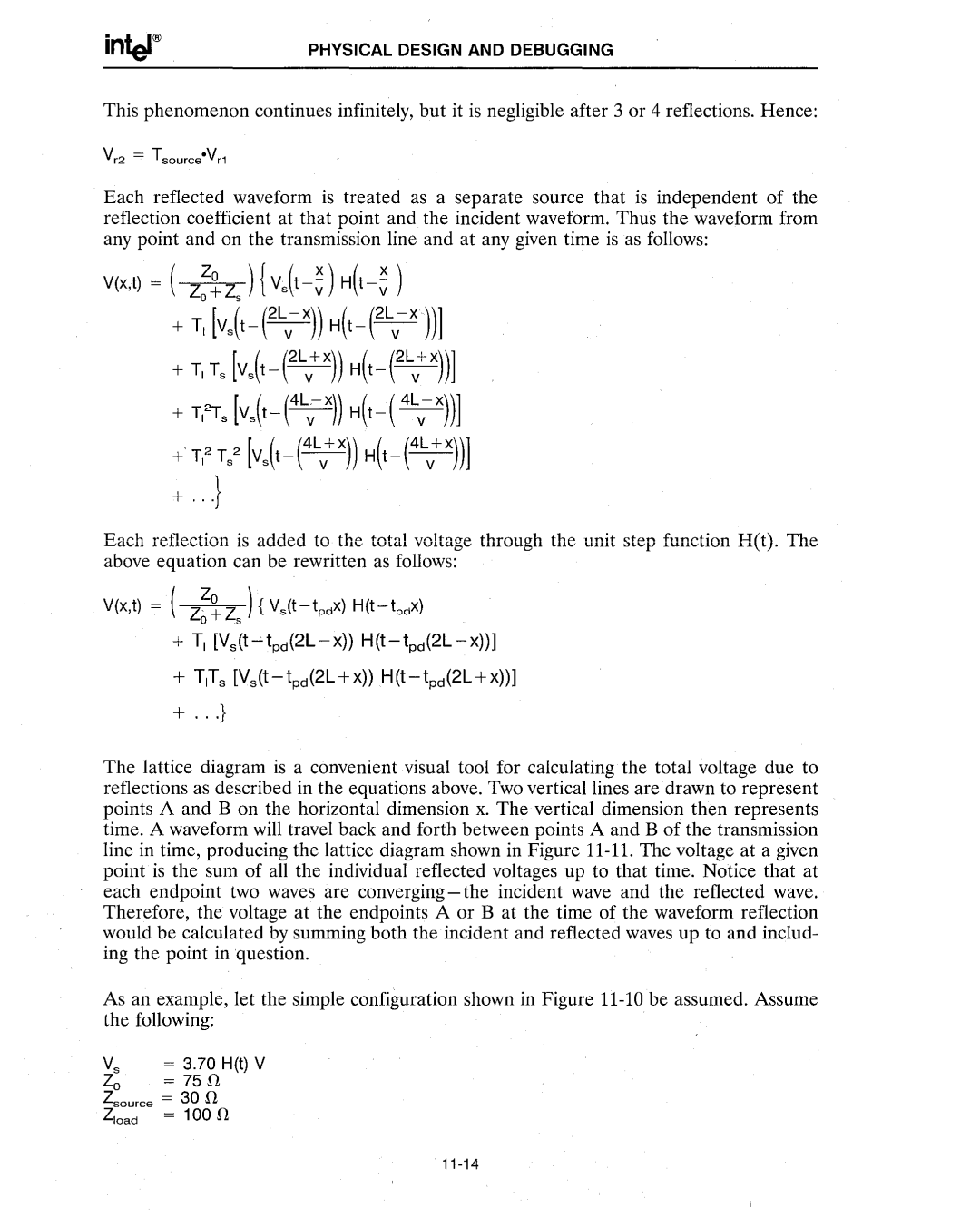
This phenomenon continues infinitely, but it is negligible after 3 or 4 reflections. Hence:

Each reflected waveform is treated as a separate source that is independent of the reflection coefficient at that point and the incident waveform. Thus the waveform from any point and on the transmission line and at any given time is as follows:

Each reflection is added to the total voltage through the unit step function H(t). The above equation can be rewritten as follows:

V(x,t) = ( Z~~Zs) {Vs(t-tpdX)H(t-tpdx)

+TI [Vs(t-'tpd(2L-x))H(t-tpd (2L-x))]

+TITs [Vs(t-tpd(2L+x)) H(t-tpd(2L+x))]

+...}

The lattice diagram is a convenient visual tool for calculating the total voltage due to reflections as described in the equations above. Two vertical lines are drawn to represent points A and B on the horizontal dimension x. The vertical dimensioll then represents time. A waveform will travel back and forth between points A and B of the transmission line in time, producing the lattice diagram shown in Figure 11-11. The voltage at a given point is the sum of all the individual reflected voltages up to that time. Notice that at each endpoint two waves are converging - the incident wave and the reflected wave. Therefore, the voltage at the endpoints A or B at the time of the waveform reflection would be calculated by summing both the incident and reflected waves up to and includ- ing the point in question.

As an example, let the simple configuration shown in Figure 11-10 be assumed. Assume the following:

Vs	= 3.70 H(t) V
Zo	= 75!1
Zsource	= 30 !1
Zioad	= 100 !1

11-14